


Introduction: Three Decisions to Make Before Adopting Factory Energy Anomaly Detection AI
For Japanese-owned factories in Thailand considering factory energy anomaly detection AI, we think the following situation is common. There is a power monitoring screen. Values are being collected every 15 minutes. And yet nobody can look at the chart and say whether today’s consumption is high or low. Because consumption swings with production volume and outdoor temperature, a simple fixed threshold produces nothing but false alarms, and before long nobody looks at the alerts at all.
2026 is also a year in which several reasons to revisit the “quantity” of electricity overlapped. According to a report by The Nation on 23 July 2026, the Energy Regulatory Commission (ERC) approved an Ft of 16.23 satang/kWh for the September to December 2026 billing period, and the average tariff was held at 3.95 baht/kWh (excluding VAT). A report in the same paper on 12 August 2026 said that the average for September billing would be about 3.89 baht/kWh (excluding VAT), because the cost of public street lighting was removed from the tariff. However, this reduction was reported as applying to “general users”, and the article does not say whether it applies to industrial users or how it will be handled from October onward. Also according to The Nation, in a report on 1 July 2026, Thailand’s total electricity consumption in January to March 2026 was 51,127 GWh, up 4.9% year on year; industrial use rose 2.2% and accounted for 42.3% of the total.
The other change is the shutdown of general-purpose cloud “anomaly detection APIs”. According to the official AWS page, support for Amazon Lookout for Equipment ended on 7 October 2026. According to Microsoft Learn, Azure AI Anomaly Detector was retired on 1 October 2026. Anyone who had built monitoring on top of these services now has to rebuild it.
So, if you bring in AI, will energy waste be found automatically? In this article, we take the view that when you introduce AI for energy anomaly detection in a factory, what you decide first is not the name of the algorithm but the following three things.
- What you compare against to call something an anomaly: Look not at consumption itself, but at the gap from an “expected consumption (baseline)” derived from relevant variables such as production volume, product mix and outdoor temperature.
- Separate the model-fit criteria from how alerts are issued: A model that predicts well and alerts that are useful are separate design items. Every alert gets a person responsible for confirming the cause and a deadline.
- Settle revision and portability in the contract: Write into the RFP (request for proposal) the conditions for revising the baseline, the explanatory variables and how data and models can be taken out, then verify them in the PoC and in FAT/SAT (factory acceptance test and site acceptance test).
Below, we check the grounds for these three points in this order: the U.S. Department of Energy (DOE) guidance on ISO 50001, material citing ASHRAE Guideline 14, a public benchmark, public documents from major products, and Thai regulations. Finally, we turn them into RFP and acceptance test items.
What Is Energy Anomaly Detection AI? The Target Is “Waste” More Than “Failure”
Energy anomaly detection AI continuously watches the consumption of electricity, compressed air, steam, gas and so on, and flags “usage that is different from usual”. What this article mainly deals with is not so much early signs of equipment failure as the energy waste that slips into day-to-day operation. Examples include equipment left running on holidays or during lunch breaks, standby power that does not drop after production ends, compressed air consumption that stays high at night, and drifting set points for air conditioning or cooling water.
Anomaly detection for early signs of equipment failure uses per-machine signals such as vibration, temperature and current waveforms, and its purpose is to “stop the machine before it breaks”. Energy anomaly detection, by contrast, compares the consumption of a factory or a group of equipment with “the amount that is reasonable given production and weather”, and its purpose is to find “the time periods and places where extra energy is being used”. Even under the same label of “anomaly detection AI”, the data used, the judgment criteria and the people who receive the alerts are different.
The overall picture of which area to start with when applying anomaly detection AI in a factory is covered in Anomaly Detection AI 2026 | Where to Start Among Five Areas. This article is the implementation-level detail for the energy area. For the systems that anomaly detection assumes, such as how to choose metering points and the cost of visualization, see Energy Monitoring System Cost and Rollout for Thai Factories.
Even in research, deciding “what to call an anomaly” is not simple. A review by Himeur et al. (Applied Energy, 2021) broadly surveys AI-based anomaly detection in building energy consumption and lists among the open challenges that “there is no precise definition of anomalous power consumption”, and that annotated datasets and unified evaluation metrics are lacking. The main subject of that review is residential sub-meters and smart sensors, but we think the situation is the same in factories. That is exactly why the adopting side needs to define anomalies first.
There is also research that targets factories. A paper by Mendia et al. (Expert Systems, February 2024) reports a tool that characterizes a factory’s “normal production and energy behavior” without supervision and in a form people can understand, monitors energy consumption and production together to detect anomalies and inefficiencies, and identifies causes at the line, process and machine level. It was evaluated on data from the automotive parts maker GESTAMP and is reported to have performed better than the unsupervised and semi-supervised methods it was compared with. Because performance figures are not given in the abstract, this article does not quote any. What is worth noting is the design direction: look at energy and production together, and present causes in a form people can understand.
Why Consumption Alone Cannot Reveal Anomalies: Normalizing EnPIs
You cannot judge from a consumption chart alone because consumption moves not only with “waste” but also with “how busy production is” and “how hot it is”. It is natural for consumption to rise on days with high production, and calling that an anomaly produces a false alarm. Conversely, it is the days when production is low but consumption does not fall much that may be hiding waste.
ISO 50001:2018 is a framework for tracking improvement through energy performance indicators (EnPIs) and the energy baseline (EnB). According to the guidance in the U.S. DOE “50001 Ready Navigator” (published by Lawrence Berkeley National Laboratory), which corresponds to ISO 50001:2018, an EnPI can take the form of “a single metric”, “a ratio (intensity)” or “a numerical model that takes one or more relevant variables into account”. It also states that where relevant variables exist, energy consumption itself cannot be used as the EnPI, and the EnPI should be normalized. The criteria for judging whether a relevant variable “significantly affects” energy are said to be decided by the organization.
Normalization here means comparing after evening out differences in conditions such as production volume and outdoor temperature. Intensity (kWh per piece and so on) is the simplest form of normalization, but where part of the consumption occurs regardless of production volume, such as standby power, it has the quirk of making intensity look worse on days with less production. A regression model with several relevant variables is one way to compensate for that quirk.
The role of EnPIs and the EnB in ISO 50001, and the path from visualization to payback, are explained in ISO50001 Energy Management 2026: Payback Starts With Power Visibility. Note that ISO 50006:2023 (2nd edition, May 2023) provides guidance on establishing, using and maintaining EnPIs and the EnB, and is said to be usable whether or not ISO 50001 is in place. However, this article has not checked the specific statistical criteria in its clauses and does not deal with them.
We should also state where this article draws its line. Measuring and verifying “how much was saved” after an energy-saving measure, and accepting it, is the job of M&V (Measurement and Verification). ISO 50015:2014 is the standard that sets out general principles and guidance for this, and it is said to be usable in combination with protocols such as IPMVP. How to accept the savings from a measure through M&V is left to Factory Energy-Saving Measures: From Metering to Verified Savings. This article is not about before and after a measure, but about finding waste and anomalies in day-to-day operation. The tools (baseline, regression, normalization) are shared, but the purpose and the frequency of judgment are different.
How to Build a Baseline (Expected Consumption) Model
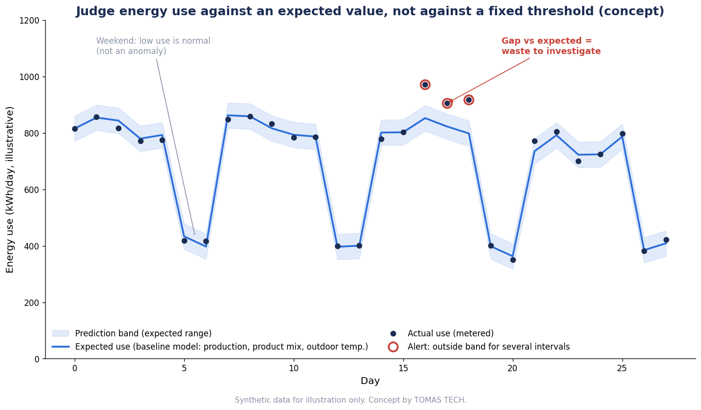
At the heart of energy anomaly detection is a model that outputs expected consumption: “under these conditions, this is about how much should be used”. When the gap between the measured value and the expected consumption is large, and that gap goes beyond the range that is statistically plausible, it becomes an anomaly candidate.
From Regression to Machine Learning
The most basic form is a linear regression with production volume and outdoor temperature as explanatory variables. Product mix, operating shift, day of the week, holiday flags and so on are then added. Where relationships are not linear, or where variables interact in complex ways, machine learning such as tree-based methods or neural networks may be used.
A systematic review of ISO 50001 EnPIs and computational models, published in the MDPI journal Algorithms, screened 2,691 of 5,442 records and analyzed 283 in detail. According to the review, research has shifted from conventional indicators and normalized baselines toward modeling with regression analysis, machine learning and deep learning. Intelligent methods make “dynamic baselines” and “early detection of abnormal consumption patterns” possible, while data quality, model interpretability and methodological standardization remain challenges. Its conclusion is that intelligent methods should transform EnPIs rather than replace them.
In this article, we think it is better to prioritize whether people on the shop floor can explain “why the expected value is what it is” over how new the algorithm is. If the person who receives an alert cannot look at the production volume or temperature behind the expected value and agree that “yes, today should have been lower”, the alert will not lead to an on-site check.
Choosing Explanatory Variables
Candidate explanatory variables include production volume (pieces, weight, stroke count and so on), product type or product mix, operating hours or shifts, outdoor temperature (and humidity if needed), and holiday and planned-shutdown flags. When choosing, check the following.
- Is it a variable that actually drives consumption? Confirm it both from shop-floor experience and from the relationship in the data.
- Can it be obtained for the same period and at the same granularity as consumption? The regression guide from BPA (the U.S. Bonneville Power Administration) also states that explanatory and dependent variables should be measured over the same periods.
- Who provides it, from which system, and by when? If production volume lives in MES or ERP and is only finalized daily, anomaly judgment will also be daily.
The Baseline Period Should Cover the Full Range of Operating Conditions
BPA’s “Regression for M&V: Reference Guide” (Version 3.0, May 2024) states that baseline period data should “cover” the full range of operating conditions. Where weather has an effect, 12 or 24 months is typical, and it explains that data from October to April alone does not cover peak summer conditions, so predictions would fall outside the range. It also says that in production environments, a period in which “production consistency” was maintained needs to be chosen.
Where air conditioning or chiller load is large in a Thai factory, we think that without a period covering the hot, rainy and dry seasons, expected values will miss as soon as the season changes and false alarms will increase. If you need to go live quickly, a realistic approach is to label a model built on a short period as “provisional” and plan to rebuild it once a full seasonal cycle has passed.
15-Minute Data and Autocorrelation
As discussed later, tariffs for large customers in Thailand are set by 15-minute average demand. We think that aligning the collection granularity to 15 minutes makes it easier to reconcile with billing. How to make 15-minute data collection trustworthy is explained in Power Meter Data Collection: An RFP for Trusted 15-Minute Data.
Fine granularity does, however, come with statistical caveats. BPA’s guide says that higher-frequency data tends to make it easier to reduce the uncertainty of savings, but that with hourly or finer data, autocorrelation (successive values being similar) distorts statistical calculations and requires additional treatment. According to the same guide, Annex D of ASHRAE Guideline 14 states that autocorrelation can be ignored if the autocorrelation coefficient ρ is below 0.5. When 15-minute data is used for anomaly judgment, a two-tier approach is conceivable, such as producing expected values in 15-minute steps while also checking the statistical evaluation on a daily or hourly basis.
Guide Values for Model Fit: How to Read ASHRAE Guideline 14
For “how well” a baseline model fits, there are statistical guide values that have been used in the M&V field. The best known are CV(RMSE) (the size of the prediction error divided by the mean) and NMBE (prediction bias).
| Metric and guide value | What it means | Source and conditions |
|---|---|---|
| CV(RMSE): up to 20% | Upper limit for a regression baseline of energy use when the reporting period has less than 12 months of data | ASHRAE Guideline 14-2014 (as cited in an EVO M&V Focus article, October 2022) |
| CV(RMSE): up to 25% | Upper limit for energy use when savings are calculated with 12 to 60 months of data | Same as above |
| CV(RMSE): less than half the expected savings rate | Recommended by EVO for linear regression. IPMVP sets the CV(RMSE) of each meter below 50% of the expected savings rate | The same article |
| Bias (net determination bias error): below 0.005% | An energy model is accepted if this condition is met | ASHRAE Guideline 14-2014 (as cited in the BPA guide) |
| R²: above 0.75 | Rule of thumb when using monthly billing data | BPA guide (a rule of thumb, not a requirement of the standard) |
| Autocorrelation coefficient ρ: below 0.5 | Autocorrelation can be ignored | ASHRAE Guideline 14 Annex D (as cited in the BPA guide) |
There are three caveats when reading this table.
First, the CV(RMSE) values of 20% and 25% listed here are guide values for the fit of a regression baseline. They are wording from ASHRAE Guideline 14-2014 as quoted in a contributed article from EVO (Efficiency Valuation Organization). Because the ASHRAE original is paid, this article has not checked the original text. In addition, according to the BPA guide, the latest edition is ASHRAE Guideline 14-2023, and we have not been able to confirm whether the values changed in the 2023 edition.
Second, these are not pass criteria for AI anomaly detection. The purpose of M&V is to correctly estimate savings over a certain period. The purpose of anomaly detection is to find large deviations in individual time periods. Even if the overall CV(RMSE) of a model is small, it is possible to have too many alerts or to miss the anomalies that matter. Conversely, if the model fit does not meet the guide values (for example, if CV(RMSE) exceeds the guide value), there may be missing explanatory variables or a problem with the data, and we think that should be fixed before issuing alerts.
Third, the author of the EVO article says that many experts put more weight on CV(RMSE) than on R². Because R² tends to come out high when consumption varies widely, it is important not to judge a model as “fitting well” on R² alone.
In the RFP, we recommend having the vendor state “over which period of data, which metrics, and in which unit (15 minutes, hourly, daily) it will report”, and making sure those values are in a form your company can check itself.
Data Preparation and Quality: Do Not Let the Model Learn Anomalies as Normal
The quality of a baseline model is determined by the quality of the data used to train it. BPA’s guide sets out the following steps for data cleaning.
- Outliers: Investigate the cause, and record and then exclude those that are genuinely abnormal, such as equipment failures, unusual closures or meter malfunctions.
- Non-routine events: Adjust for retrofits, expansions, additions or removals of equipment, changes to operating schedules and so on.
- Missing data: For large gaps, look for the cause or for substitute data (such as a nearby weather station). Fill a small number of gaps with, for example, the average of adjacent values, and interpolate with a regression model when there are many.
- Duplicates: Interval data is prone to duplication, so remove duplicates.
The same guide says cleaning should be done for both the baseline period and the reporting period. Applied to anomaly detection, we think that if periods of air leaks or nights when equipment was left running remain in the historical data used for training, the model will learn them as “normal”. The LEAD1.0 paper also notes that the outlier annotations removed by top Kaggle participants were incomplete. Picking out past anomalies is unglamorous work, but it cannot be skipped.
EVO, which runs IPMVP, distinguishes routine adjustments (aligning conditions, through regression and the like, for factors expected to change routinely) from non-routine adjustments (adjustments when factors assumed not to change have affected energy use for reasons other than the energy-saving measure). Treating changes in production volume or temperature as “routine” ones that the model absorbs, and line additions or equipment removals as “non-routine” ones recorded outside the model, makes the baseline revision discussed later easier to organize.
How to plan the data dictionary, time synchronization and the handling of missing data is covered in detail in Energy Management System: ISO/DIS 50012 Data Planning. For how to build sensor and communication data loss into acceptance criteria, see Factory Sensor Data Loss Prevention: RFP, FAT and SAT Acceptance Criteria. For anomaly detection, you also need to decide whether missing data itself should trigger an alert. This is so that a stopped meter reading zero is not mistaken for “a large energy saving”.
Alert Design: Decide It Separately From Model Fit
Once the model is built, the next step is how alerts are issued. This is the second point of the backbone of this article. The model-fit criteria and the alert conditions are decided as separate design items.
Use the Prediction Interval to Define the “Plausible Range”
According to BPA’s guide, a prediction interval is “the range in which a single observation should fall”, and it is wider than the confidence interval of the mean. We think it is natural to use this prediction interval when deciding how far a measured value for an individual time period must be from the expected value to be considered abnormal. Falling outside the prediction interval does not always mean an anomaly, but it does make the point a candidate for “a deviation that is hard to explain by model error”.
Combine Duration, Cost and Priority
If you notify every time a single 15-minute value falls outside the prediction interval, there will be far too many alerts. In practice, combining conditions such as the following is conceivable.
| Design item | What to decide | Approach (this article’s view) |
|---|---|---|
| Size of deviation | Whether it is outside the prediction interval, and how far it is from the expected value | Only deviations that are hard to explain by model error become candidates |
| Duration | How many consecutive intervals, or how many hours, before notifying | A sustained deviation is more likely to be waste than a momentary one |
| Conversion to cost or quantity | Whether to express the deviation in kWh or money | Makes it easier for the shop floor to prioritize. Set the unit price yourself from your contract and bills |
| Priority | Urgent, same day or weekly categories | Bundle small, persistent deviations into a weekly review |
| Recipients | Who is notified and through which channel | Assign owners by equipment or area, and also consolidate to the PRE |
| Confirmation deadline | By when the cause must be confirmed | Alerts without deadlines stop being looked at |
| Suppression conditions | Whether to mute during planned shutdowns, trial runs or equipment replacement | Do not alert on known events |
When converting to money, set the unit price from your own contract category and actual bills. The average tariffs that are reported are averages for general users, not your company’s own tariff.
Prevent Alert Fatigue by “Measuring the Count”
In the process control field there are alarm management standards such as ISA-18.2 and EEMUA 191, and the idea of setting guide values for the number of alarms a single operator receives has been introduced in several secondary sources. These are guide values for operator alarms, not criteria for energy anomaly alerts. Even so, we think the idea of “designing the number of alerts, measuring the actual number, and revising the conditions if there are too many” can be borrowed as it is.
The public benchmark paper also cites as a challenge that, because labeled data is unavailable, unsupervised methods are widely used and false positives become frequent. In a news article on energy management, ABB explains that because equipment efficiency changes with age, manual alert thresholds need to be updated continuously. Whether thresholds are set by hand or AI generates the expected range, you need a mechanism to review the number and content of alerts every week.
Assign a Person and a Deadline to Confirm the Cause
An energy anomaly alert, on its own, is only a “waste candidate”. Only after someone goes to the floor and confirms what was happening can you tell whether it is waste, legitimate use, or a metering problem. In this article, we recommend an operation in which every alert is always given “a person who confirms it” and “a deadline for confirmation”, and the result of the confirmation is recorded. We think an alert with no owner will not lead to results, however accurate it is.
What a Public Benchmark Tells Us: Hits Are Mostly Right, but Many Anomalies Are Missed
How usable are off-the-shelf AI methods for energy anomaly detection? One public benchmark is LEAD1.0 (Gulati & Arjunan, arXiv 2203.17256, 30 March 2022). Let us check the conditions first.
- The subject is 1,413 electricity meters in commercial (non-residential) buildings, with one year of hourly values for 2016. It is not factory data.
- Point anomalies and contiguous (collective) anomalies were manually labeled on data from the ASHRAE Great Energy Predictor III (Kaggle, 2019) (about 100 person-hours). Anomalies were 199,640 out of 12,060,910 points (missing values not counted).
- The evaluation is “whether a 24-hour window is anomalous or not”. The methods are 8 off-the-shelf unsupervised methods from PyOD. The metrics are Precision (of the items judged anomalous, the share that were truly anomalous), Recall (of the true anomalies, the share that were caught) and F1 (the harmonic mean of the two).
The results are as follows (Table 1 of the paper).
| Method | F1 | Precision | Recall |
|---|---|---|---|
| KNN | 0.431 | 0.902 | 0.284 |
| LOF | 0.426 | 0.900 | 0.281 |
| CBLOF | 0.425 | 0.900 | 0.277 |
| Feature Bagging | 0.424 | 0.899 | 0.279 |
| MCD | 0.422 | 0.901 | 0.276 |
| OCSVM | 0.421 | 0.899 | 0.276 |
| Isolation Forest | 0.413 | 0.895 | 0.270 |
| HBOS | 0.397 | 0.896 | 0.258 |
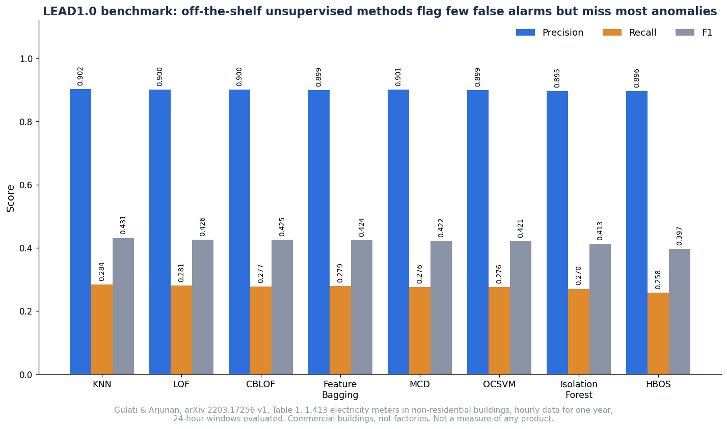
Under these conditions, all 8 methods had high Precision of 0.895 to 0.902, while Recall stayed at 0.258 to 0.284, and F1 was 0.431 even for KNN, the highest. In other words, the result is that “the windows judged anomalous were mostly correct, but many of the anomalies labeled by people were not caught”. The authors themselves note that this is a limited benchmark.
This article draws two points from this result.
First, do not evaluate AI by a single number. When someone says “the accuracy is high”, the meaning is completely different depending on whether it is Precision, Recall or F1. Confusing Precision with F1 leads to a badly wrong evaluation.
Second, simply applying off-the-shelf unsupervised methods as they are can result in many missed anomalies. After LEAD1.0, there have been studies that tried GANs or per-cluster models on the same data, but because the number of buildings, the unit of evaluation and whether the method was supervised all differ, their values cannot be lined up and compared side by side. For use in factories, we think the premise is to combine a baseline that includes factory-specific explanatory variables such as production volume and product type with an operation in which people confirm the alerts.
Hourly values from commercial buildings and 15-minute values from factories behave completely differently. Please do not read the values in this table as what you can expect in a factory. Checking with your own data, using past events your company already knows about, is the role of the PoC described in the following sections.
How the Major Products Describe Themselves
Below, we organize, in alphabetical order of company name, how public documents for major products describe their functions related to expected energy values and alerts. This table is not a comparison of strengths or a recommendation, but a way to see “what kind of mechanism each is described as”. We could not find public pricing for any of them.
| Company and product (source) | Main functions according to the company’s description | Notes on verification |
|---|---|---|
| ABB (news article on AI/ML for energy management) | According to the company, AI anomaly detection generates an expected range of energy consumption from history and retrains each time new data comes in | Confirmed from a search result excerpt. Product name and publication date not verified |
| Mitsubishi Electric EcoAdviser (official product page) | According to the company, there are two versions: a “limited-function version” (management) and an “AI diagnosis version” (analysis, diagnosis, verification and monitoring). Its proprietary AI automatically extracts energy losses from “five key energy-saving perspectives” (time loss at equipment start-up and shutdown, utility time loss, energy intensity, and ratio of production loss time). Factors such as day of week, start-up time and production count are judged automatically. Automatic monitoring of energy losses uses AI monitoring and fixed monitoring against target values | AI monitoring requires about 30 days of past data. The dashboard monitoring panel covers 10 metering points and updates once a day |
| Schneider Electric EcoStruxure Power Monitoring Expert (product help) | According to the company, it builds models of equipment and processes and displays the model-based expected consumption, the measured value and the difference between them (delta). For intensity trends, normalization data such as production volume and temperature is imported via ETL, OPC or CSV | The help text itself could not be retrieved; confirmed from search result excerpts |
| Siemens SIMATIC Energy Manager PRO / Energy Analytics (annex to a third-party audit certificate) | According to the annex, setting EnPIs, dependency analysis and regression analysis, threshold setting for early warning, determining relevant variables and static factors, and managing improvement actions have been confirmed | An official description of an AI anomaly detection function itself could not be confirmed |
Some additions to the table. According to Mitsubishi Electric’s official page, EcoAdviser manages electricity, water, compressed air, gas and heavy oil in one place and can manage energy intensity. In diagnosis, it is described as showing an estimate of the improvement effect in monetary terms and reflecting the user’s evaluation in subsequent runs. A related Schneider Electric application (Energy Modeling & Verification) is described as analyzing consumption against a baseline that takes into account drivers such as outdoor temperature, occupancy and productivity. According to the annex to Siemens’ certificate, the components covered by the certificate support compliance with ISO 50001 requirements such as 6.4 (EnPI) and 6.5 (EnB), and SIMATIC Energy Manager PRO and Energy Analytics support compliance with requirements such as 4.2.4 of ISO 50006.
What the table shows is a skeleton common to the companies’ descriptions: take in relevant variables (drivers), build an expected value, show the gap from the measured value, and notify through thresholds or expected ranges. Whether it is called “AI” or “regression”, we think the idea is the same as the “look at the gap from expected consumption” described in point 1 of this article’s backbone. The differences lie in which variables can be imported and how often, how far the basis for the expected value is shown, and how retraining can be controlled. These cannot be judged from each company’s documents alone, so they are checked in the RFP and PoC. Please also check local support arrangements and the screen languages individually with each company.
Cloud Anomaly Detection Services That Have Ended
Not included above are cloud services that ended in 2026. These are not current options; they are presented as examples of “what happens when a service ends”.
According to the official AWS page, support for Amazon Lookout for Equipment ended on 7 October 2026, after which the console and resources can no longer be accessed. According to the document history of the user guide, it had stopped accepting new customers from 17 October 2024.
According to Microsoft Learn, new Azure AI Anomaly Detector resources could no longer be created after 20 September 2023, and the service was retired on 1 October 2026. As migration paths, Microsoft Fabric, which integrates the open-source microsoft/anomaly-detector, or the open-source version itself are suggested.
In both cases, there was a period of years between the halt to new sign-ups and the shutdown. Even so, factories that had built their monitoring on such services are forced to move their models, training data and alert conditions somewhere else. This is why point 3 of this article’s backbone recommends writing “taking out data and models when a service ends” into the RFP.
Conditions and Records for Revising the Baseline (Retraining)
A baseline is not finished once it is built. When equipment is replaced, the level of consumption itself changes. This is the first half of the third point of the backbone.
According to the DOE guidance, the EnB is revised in the following cases: (1) when the EnPI no longer accurately reflects the organization’s energy performance, (2) when there have been major changes to static factors, processes, operating patterns or energy systems, and (3) in accordance with a predetermined method. It also states that records of changes and updates to the EnB must be retained.
Translated into factory examples, situations like the following become triggers for revision.
- Energy-saving measures such as replacement with high-efficiency compressors or chillers, or conversion of lighting to LED
- Addition or removal of lines, or extension of buildings
- Major changes in product mix (more or fewer energy-intensive products, for example)
- Changes to the shift system or holiday calendar
- Addition of metering points, or replacement of meters or CTs
ABB, on the other hand, describes an approach in which the AI retrains each time new data comes in so the baseline follows along. Automatic tracking makes it easier to keep up with equipment aging. However, we think there is also a risk that slowly progressing waste (such as gradually increasing air leaks or fouling of heat exchangers) gets absorbed as “the new normal”. This is not a claim confirmed in a source but an inference by this article, and that is precisely why it is important to keep a record of “when, triggered by what, and with whose approval the model was retrained”.
In this article, we recommend deciding retraining in the following two categories.
- Periodic retraining: Performed on a predetermined cycle, such as once per seasonal cycle. This corresponds to (3), “a predetermined method”, in the DOE guidance.
- Event-driven revision: Performed when one of the changes listed above occurs. This corresponds to (2).
In either case, compare the model fit (the metrics in the previous section) before and after retraining, and record the reason for the change and the approver. If the anomaly detection baseline is changed arbitrarily while the effect of an energy-saving measure is being evaluated through M&V, there is a risk of inconsistency with the savings evaluation. We think it is safer to manage both in the same team, or at least to have a mechanism for sharing changes.
Cause Confirmation Flow: From Alert to Action and Record
What turns alerts into results is the cause confirmation flow. In this article, we organize it into the following six stages.
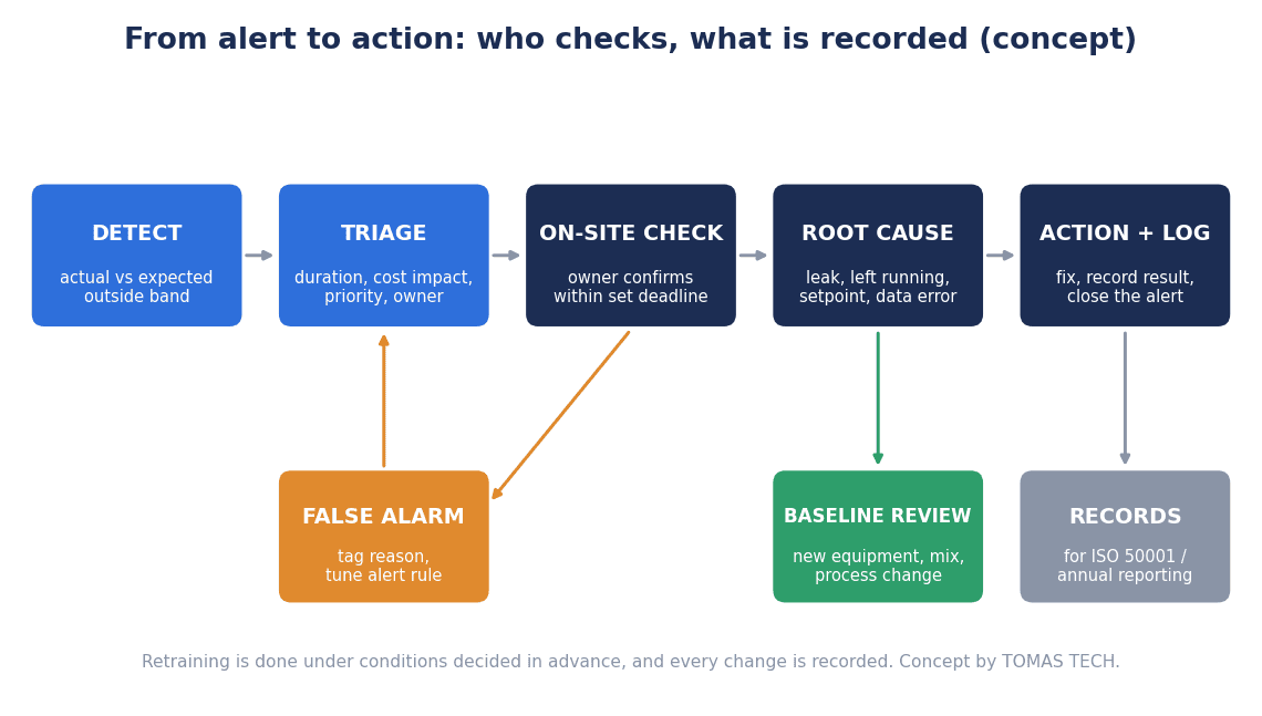
- Detection (DETECT): The gap from the expected value exceeds the defined conditions (prediction interval, duration and so on).
- Triage (TRIAGE): Make a first judgment on screen as to whether it is a known event such as a planned shutdown or trial run, a metering fault (missing data, zero values, duplicates), or a genuine operational anomaly.
- On-site check (ON-SITE CHECK): The person in charge checks on site by the deadline.
- Root cause classification (ROOT CAUSE): Classify into categories such as equipment left running, set-point drift, leaks, equipment deterioration, errors in production data and model errors.
- Action (ACTION): Fix what can be fixed on the spot, and register anything that requires capital investment as an improvement project.
- Record and retraining decision (LOG / RETRAIN?): Record the result and decide whether the baseline needs to be revised.
Where to check for the cause depends on the system that raised the alert. For example, if compressed air consumption does not fall at night or on holidays, air leaks and compressor sequencing are where to look. Revising compressor sequencing is covered in AI Compressor Sequencing in Thai Factories: Selection and Acceptance Guide. If consumption in the air conditioning or cooling system is high for the outdoor temperature, the operating state of the chillers is where to look. For chiller metering points and how to approach monitoring, see Factory Chiller Monitoring: Sensors, kW/ton and FAT/SAT.
What matters in this flow is to always include “model error” and “production data error” in stage 4, “root cause classification”. We think that once anomaly detection is in operation, a certain share of alerts will turn out not to be waste but to stem from missing production volume entries or operating conditions the model does not know about. If you record these, you can use them to add explanatory variables or improve data integration. If you do not, the same false alarms will repeat and you will lose the trust of the shop floor.
We recommend recording at least “date, time and system of the alert”, “gap between expected and measured value”, “who confirmed it and when”, “cause category”, “action and completion date” and “whether retraining is needed”. As described later, at designated factories in Thailand the PRE is responsible for regularly monitoring equipment efficiency, and we think these records can also serve as evidence of that activity.
Thailand-Specific Issues: Designated Factories, 15-Minute Demand and Ft
Designated Factory Criteria and PRE Duties
Under Thailand’s Energy Conservation Promotion Act (ENCON Act), factories above a certain size are treated as “designated factories”. According to a presentation by the Department of Alternative Energy Development and Efficiency (DEDE) dated 28 February 2023, Group 1 designated factories are those with a contracted electricity meter capacity of 1,000 to 3,000 kW, transformers of 1,175 to 3,530 kVA, or annual energy consumption of 20 to 60 TJ, and Group 2 covers those above that. Those with an electricity meter below 1,000 kW, transformers below 1,175 kVA and annual consumption below 20 TJ are classified as not designated factories (SME).
According to the same material, designated factories appoint a Person Responsible for Energy (PRE). Group 1 needs at least one (C-PRE), and Group 2 needs at least two, one of whom is a Senior PRE (S-PRE). They operate an energy management system in line with the regulations, and submit an annual report, audited and certified by an energy auditor, to DEDE during March each year. The PRE’s duties include regularly maintaining and monitoring the efficiency of machinery and equipment, making improvements in line with energy conservation measures, and assisting the owner in operating the energy management system.
When considering who should receive energy anomaly alerts, we think the PRE is one natural recipient. However, if all alerts are concentrated on a single PRE, on-site checks will not keep up. A realistic division of roles is for the PRE to handle aggregation and trend review, and for the equipment owners in each area to handle individual on-site checks.
Tariffs Are Set by 15-Minute Average Demand
According to PEA’s tariff schedule (English unofficial translation, May 2023 edition), the large category (Schedule 4 Large General Service) covers businesses, factories and so on whose maximum 15-minute average demand is 1,000 kW or more, or whose average consumption over the last three months exceeds 250,000 kWh per month. The medium category (Schedule 3) is 30 kW or more and below 1,000 kW. Because demand charges are set by the maximum 15-minute value, we think that keeping 15-minute values as the minimum granularity for anomaly detection makes it easier to reconcile with billing. Note that the unit prices in that tariff schedule are 2023 values and do not reflect later revisions, so this article does not quote them. How to approach control that limits peak demand is explained in Demand Control 2026: In Thailand the Peak Is Set in 15 Minutes, Not 30.
Use Ft and Tariff Figures Exactly as Reported
As mentioned at the start, it has been reported that the Ft for the September to December 2026 billing period is 16.23 satang/kWh and that the average tariff was held at 3.95 baht/kWh (excluding VAT). The figure of about 3.89 baht for September billing was reported as applying to general users, and we have not been able to confirm whether it applies to industrial users or from October onward. When converting deviations into money, please use your own contract category and actual bills rather than reported averages. Even while unit prices move, we think that if you track deviations in the “quantity” of kWh as gaps from expected values, you can separate tariff changes from the occurrence of waste.
Subsidies and Incentives Need to Be Checked Individually
Regarding subsidies for energy-saving equipment and BOI investment incentives, the research for this article found no material confirming that energy monitoring or anomaly detection software is eligible. Because schemes can be revised, if you are considering using one, you need to check the latest conditions with DEDE or the BOI.
Items to Include in the RFP
Now we turn the issues so far into RFP items. This is the second half of the third point of the backbone. How to put together an RFP and FAT/SAT for energy monitoring in general is explained in Thailand Factory Energy Monitoring RFP: FAT/SAT and PoC. Here we focus on items specific to anomaly detection.
| Item | What to write in the RFP | Why it needs checking |
|---|---|---|
| Scope and metering points | Target buildings, lines and utility systems, a list of metering points, and whether non-electric utilities (compressed air, steam, gas, water) are included | Determines whether the cause of an anomaly can be narrowed down to a system |
| Granularity | Collection granularity (such as 15 minutes), the granularity at which expected values are produced, and the granularity at which alerts are judged | Aligns the tariff logic with statistical treatment |
| Explanatory variables | Variables to import, such as production volume, product type, operating hours, outdoor temperature and holiday flags, their sources (MES, ERP, weather data) and import frequency | They form the basis of expected consumption |
| Baseline period and revision conditions | Training period, coverage of operating conditions, periodic retraining cycle, conditions for event-driven revision, and approval procedure | Corresponds to EnB revision and retention of records |
| Fit reporting | Metrics such as CV(RMSE), bias and R², the period and unit of calculation, and reporting frequency | Lets your company check the state of the model itself |
| Data cleaning | Treatment of outliers, non-routine events, missing data and duplicates, and records of excluded periods | Prevents the model from learning anomalies as normal |
| Alert conditions and recipients | Prediction interval, duration, cost conversion, priority and suppression conditions, notification channels and recipients, and who can change the conditions | Manages the number and content of alerts |
| Confirmation owners and workflow | Confirmation owners and deadlines, list of cause categories, records of action and completion, and monthly count of alerts | Builds the practice of people confirming causes into the system |
| Explanation of expected values | Whether, for each alert, the values of the variables behind the expected value can be displayed | Lets the shop floor accept the alert and act on it |
| Ownership and portability of data and models | Ownership of metering data, trained models, model settings and explanatory variable definitions, and alert and confirmation history, plus export formats and deadlines at contract termination or service shutdown | Prepares for the shutdown of cloud services |
| Retention period | Retention periods for raw data, expected values, alerts and confirmation records | Used for annual reports and historical comparison |
| Cost breakdown | Costs for initial build, metering equipment, licenses, cloud usage, retraining and maintenance, and per additional metering point | Avoids overlooking operating-phase costs |
The item that deserves particular attention is “ownership and portability of data and models”. As we saw in the previous section, cloud anomaly detection services can end. A trained model itself cannot necessarily run in another environment, but if you at least have the explanatory variable definitions, the data and period used for training, the excluded periods, the alert conditions and the confirmation history, you can rebuild it on another system. We recommend making sure these can be received, contractually, as your company’s own property.
Designing the PoC and Acceptance Tests (FAT/SAT)
Once the requirements are fixed in the RFP, verify them in the PoC and acceptance tests. Here too, the principle is that “your company decides the pass line”. The research for this article did not find any public standard that sets numerical pass/fail criteria for anomaly detection in FAT/SAT. The following are examples of how to approach it.
Validation on Historical Data
It is efficient to run the first PoC on historical data. Build a model from data covering the seasons, apply it to a different period, and see where alerts are raised. In doing so, always include past events your company already knows about. Examples are the period when an air leak was found and repaired, a period when air conditioning was set incorrectly, and holidays when a line was left running. Record by count whether these are detected (are there any missed anomalies?) and how many alerts are raised at other times (how many false alarms?).
As the LEAD1.0 results show, Precision and Recall move independently. In the PoC, we recommend counting both “the alerts that turned out to be meaningful when checked” and “the known events that were caught”. Which one to weight more heavily depends on how many people you can assign to confirmation and on the loss when an anomaly is missed. It is important to set the pass line before the PoC starts and not to move it conveniently after it ends. Equipment Anomaly Detection PoC: 90-Day Acceptance Criteria for Thai Factories is also a useful reference on how to run an equipment anomaly detection PoC.
Testing That Includes Operations
Make not only performance but also the operational flow a subject of testing. In FAT, check that importing explanatory variables, calculating expected values, setting and changing alert conditions, notifications, entering confirmation records, and exporting data and models work as specified. In SAT, with the actual metering points connected, check the behavior when there are time offsets or missing data, suppression during planned shutdowns, and whether notifications reach confirmation owners in time.
In addition, we recommend actually performing a baseline revision once during testing. If you confirm how the fit metrics changed before and after the revision, and that the reason for the change and the approver were recorded, you will not be caught off guard when equipment is replaced in production. Likewise, it is safer to check once at the acceptance stage that data and models can be exported in the format agreed in the contract.
Frequently Asked Questions
Do You Need AI for Energy Anomaly Detection? Won’t Thresholds Do?
For equipment whose consumption does not move much with production volume or outdoor temperature, fixed thresholds can be useful in some cases. However, as the DOE guidance shows, where relevant variables exist, consumption itself cannot be used for evaluation and normalization is needed. ABB also explains that manual thresholds need to be updated continuously as equipment ages. We think what matters is not whether it is called AI or regression, but whether you are comparing against an expected value that includes relevant variables.
How Much Data Do You Need to Build a Baseline?
According to BPA’s guide, where weather has an effect, 12 or 24 months is typical, and the data needs to cover the full range of operating conditions. In production environments, choose a period in which production consistency was maintained. If you start with a short period, we recommend treating it as a provisional model and planning to rebuild it once a full seasonal cycle has passed. Note that Mitsubishi Electric explains that AI monitoring in EcoAdviser requires about 30 days of past data. The required period differs by product and purpose, so check it in the RFP.
What Is EnPI Normalization?
It means comparing energy performance after evening out differences in relevant variables such as production volume and outdoor temperature. According to the DOE guidance, an EnPI takes the form of a single metric, a ratio (intensity), or a numerical model that takes relevant variables into account, and where relevant variables exist it should be normalized. An anomaly detection baseline can be described as applying this normalization idea to daily monitoring.
What Should You Do When There Are Too Many False Alarms?
First, record the number of alerts and the confirmation results, and classify the causes. Where the fix belongs depends on whether a false alarm is caused by missing production data entries, operating conditions the model does not know about, or a metering fault. Possible measures include adding explanatory variables, adding suppression conditions for planned shutdowns, and revising the duration conditions. If you change the conditions, record the reason and the date of the change.
What Happens When a Cloud Service Ends?
Support for Amazon Lookout for Equipment ended on 7 October 2026, and Azure AI Anomaly Detector was retired on 1 October 2026. After a shutdown, models can no longer run on that service. If your company holds the explanatory variable definitions, the training data and period, the alert conditions and the confirmation history, you can rebuild on another system. We recommend deciding the ownership and export formats of these in the RFP.
Summary
- When introducing AI for energy anomaly detection in a factory, what you decide first is not the name of the algorithm but three things: (1) what you compare against to call something an anomaly, (2) separating the model-fit criteria from how alerts are issued and running an operation in which people confirm causes, and (3) writing the revision conditions and the portability of data and models into the RFP and verifying them in the PoC and FAT/SAT.
- According to the DOE guidance, where relevant variables exist, energy consumption itself cannot be used as the EnPI, and normalization is needed. Looking at the gap from expected consumption (the baseline) is the starting point.
- The ASHRAE Guideline 14-2014 guide values for regression baselines (as cited in the EVO article: CV(RMSE) of 20% when the reporting period has less than 12 months of data, and 25% for 12 to 60 months) are guide values for model fit, not pass criteria for alerts.
- In LEAD1.0, which evaluated 8 off-the-shelf unsupervised methods on one year of hourly values from 1,413 commercial building meters, Precision was high at 0.895 to 0.902, while Recall was 0.258 to 0.284. Do not evaluate AI by a single number; count missed anomalies and false alarms separately.
- Revise the baseline under defined conditions and keep records. Cloud anomaly detection services ended one after another in 2026, so it is important to settle the portability of data and models in the contract.
TOMAS TECH is happy to help even at the stage of taking stock of your metering data or considering which variables a baseline could be built from. Please get in touch here.
References
- DEDE, “Thailand’s Energy Efficiency”, 28 February 2023 (published by NEDO, PDF) https://www.nedo.go.jp/content/100959493.pdf
- The Nation, “Power tariff held at 3.95 baht through year-end”, 23 July 2026 https://www.nationthailand.com/news/general/40068945
- The Nation, “Thailand cuts September power tariff, caps first 200 units at 3 baht”, 12 August 2026 https://www.nationthailand.com/news/general/40069705
- The Nation, “Thailand’s energy consumption rises 2.1% on 2.8% GDP growth”, 1 July 2026 https://www.nationthailand.com/business/economy/40068117
- PEA, “Electricity Tariffs”, May 2023 edition (English unofficial translation, PDF) https://www.pea.co.th/sites/default/files/documents/tariff/EN_Electricity_Tariffs_May_2023.pdf
- ISO, “ISO 50001:2018” https://www.iso.org/standard/69426.html
- U.S. DOE 50001 Ready Navigator, “Task 11: Energy Performance Indicators and Energy Baselines” https://navigator.lbl.gov/guidance/task/11
- DIN Media, “DIN ISO 50006” https://www.dinmedia.de/de/norm/din-iso-50006/384067911
- ISO, “ISO 50015:2014” https://www.iso.org/standard/60043.html
- EVO M&V Focus Issue #10, John Avina, “Relaxing CV(RMSE) requirements for Option C M&V regressions”, October 2022 https://evo-world.org/en/m-v-community/mv-focus/903-m-v-focus-issue-no-10/1338-relaxing-cv-rmse-requirements-for-option-c-m-v-regressions
- Bonneville Power Administration, “Regression for M&V: Reference Guide”, Version 3.0, May 2024 (PDF) https://www.bpa.gov/-/media/Aep/energy-efficiency/measurement-verification/3-bpa-mv-regression-reference-guide.pdf
- EVO, “NRA / NRE”, IPMVP Committee page https://evo-world.org/en/about-en/organization/ipmvp-committee/nra-nre
- Schneider Electric, “EcoStruxure Power Monitoring Expert 2023”, Use Model Report https://product-help.schneider-electric.com/EcoStruxure/Power-Monitoring-Expert-2023/content/6_operating/webapps/reports/energyanalysis/usemodel_report.htm
- Schneider Electric, “EcoStruxure Power Monitoring Expert 2023”, Create Model Report https://product-help.schneider-electric.com/EcoStruxure/Power-Monitoring-Expert-2023/content/6_operating/webapps/reports/energyanalysis/createmodel_report.htm
- Siemens, “SIMATIC Energy Manager PRO / Energy Analytics”, certificate annex (PDF) https://assets.new.siemens.com/siemens/assets/api/uuid:90799adf-4e2c-42fa-885c-082bc7cabe74/certificate-no–c-09-2020-21250307.pdf
- AWS, “Amazon Lookout for Equipment” https://aws.amazon.com/lookout-for-equipment/
- AWS, “Amazon Lookout for Equipment”, user guide document history https://docs.aws.amazon.com/lookout-for-equipment/latest/ug/doc-history.html
- Microsoft Learn, “Azure AI Anomaly Detector”, overview page https://learn.microsoft.com/en-us/azure/ai-services/anomaly-detector/overview
- ABB, “Celebrating Earth Day with AI/ML energy management innovation” https://new.abb.com/news/detail/124636/celebrating-earth-day-with-aiml-energy-management-innovation
- Mitsubishi Electric, “EcoAdviser energy-saving support application” (Japanese page) https://www.mitsubishielectric.co.jp/fa/products/software/ems/eap/index.html
- Gulati, Arjunan, “LEAD1.0”, arXiv 2203.17256, 30 March 2022 https://arxiv.org/abs/2203.17256
- Himeur et al. (review of AI-based anomaly detection in building energy consumption), arXiv 2010.04560, Applied Energy Vol.287, 2021 https://arxiv.org/abs/2010.04560
- Iturralde Carrera et al., “Intelligent Computational Modeling of ISO 50001 Energy Performance Indicators for Sustainable Energy Management Systems: A Systematic Review” (DOI 10.3390/a19070533) https://www.citedrive.com/en/discovery/intelligent-computational-modeling-of-iso-50001-energy-performance-indicators-for-sustainable-energy-management-systems-a-systematic-review/
- Mendia, Gil-Lopez, Grau, Del Ser, “A novel approach for the detection of anomalous energy consumption patterns in industrial cyber-physical systems”, Expert Systems 41(2), February 2024 https://dsp.tecnalia.com/items/f7c96e3b-ba08-4afd-9af0-19f4e6074604/full
- Emerson, “Alarm Management by the Numbers” (PDF) https://d1-live.emerson.com/documents/automation/article-alarm-management-by-numbers-deltav-en-38292.pdf


