


When a factory decides to monitor its chillers, the first decision is not the dashboard layout. It is which cooling load must be protected, where the chilled water and electricity will be measured, and who will act when a reading becomes abnormal. Sending a supply-temperature tag to the cloud alone cannot show the cooling margin at a production line, the plant’s measured efficiency, or the likely cause of an alarm. Adding sensors without defining their piping locations and the operating state of each machine will not make a kW/ton calculation useful either.
This guide takes a manufacturing team through requirements, instrumentation, commissioning and acceptance of a factory chiller monitoring system. It distinguishes process cooling from comfort HVAC and water-cooled equipment from air-cooled equipment. It combines chilled-water supply and return temperature, flow, electrical power and, where relevant, condenser-water measurements. Every numerical example below is an illustrative calculation under stated assumptions, not a promised energy saving or payback period.
Define the plant and load boundaries first
Mold cooling for injection molding, heat removal in food production, chemical temperature control and chilled water for air handlers may all use a chiller, yet the consequences of a stoppage differ. For process cooling, product quality and continuity of production often determine the acceptable temperature and response time. For HVAC, indoor conditions, occupancy and the valves and coils at air-handling units are relevant. A factory-wide average water temperature can conceal a local process problem.
Inventory each chiller’s model, rated capacity, cooling type and quantity. Map primary and secondary pumps, headers, bypasses, heat exchangers, end uses, existing BMS or PLC, electrical meters, communication protocols, P&IDs and operating hours. If water splits into several lines, distinguish total flow at the main header from flows through critical branches. When the process loop contains glycol, obtain its concentration and fluid properties before applying a water-only heat calculation. Record the design conditions behind a nameplate rating before comparing them with field operation.
For a water-cooled plant, explicitly decide whether the measured boundary includes condenser-water pumps and cooling tower fans. An air-cooled chiller has no condenser-water loop. Chiller-only efficiency and whole-plant efficiency are different measures. The U.S. Department of Energy’s FEMP purchasing guidance evaluates air- and water-cooled chillers separately and also distinguishes full-load from part-load operation [1]. That guidance illustrates why comparison conditions matter; it does not set a Thai factory’s regulatory requirements.
Before procurement, answer six questions: Which line or HVAC zone is affected by an excursion, and how quickly? Is the monitored boundary an individual chiller, a header, a production line or the entire plant? Where can staff read existing instruments, and are they calibrated? Who receives and responds to alarms outside office hours? Who may change setpoints, and does the new system actually need a control-write function? What access and shutdown windows are available for installation and tests? If these answers are uncertain, begin by reconciling drawings, equipment and existing data.
Minimum and optional measurement points
Cooling capacity comes from supply temperature, return temperature and flow measured across the same chilled-water boundary. An efficiency measure also requires electrical power for that same boundary and time. Put each proposed instrument on the P&ID before counting tags. Dividing total header cooling by one chiller’s electrical input creates a plausible-looking number with no stable meaning.
| Point | Purpose | Installation and data check |
|---|---|---|
| Chilled-water supply temperature, CHWS | Supply setpoint tracking and temperature delivered to the load | Sensor insertion and mixing location, calibration and unit |
| Chilled-water return temperature, CHWR | Load trend and ΔT | Same boundary as CHWS; identify bypass mixing |
| Chilled-water flow | Cooling-capacity calculation and low-flow detection | Meter range, straight pipe requirements, flow direction, air and glycol |
| Chiller electrical kW and kWh | Equipment efficiency and measured energy | Compressor only or whole machine; CT/PT ratios and clock |
| Run, stop, fault and setpoint | Interpret readings and alarms | Manual/automatic mode, start-up transient and missing communications |
| Pump and cooling tower fan kW | Whole-plant kW/ton | Scope of auxiliary loads and variable-speed metering |
| Condenser-water inlet/outlet temperature and flow, for water-cooled systems | Clues about heat rejection, fouling and flow | Tower and bypass arrangement; design operating limits |
Condenser-side points can be valuable, but every site need not add them on day one. Separate values retrieved from an existing controller from values measured by an independently calibrated device. A controller’s displayed “flow” can be an estimate derived from differential pressure or even a setpoint. Verify how each value is produced, its unit and its update rate. Trane’s chiller plant control overview provides useful context for considering equipment and system operation as a whole [4]; actual sensing and control must follow the equipment documents and site conditions.
A sensor at the chiller connection answers a different question from a sensor at a common supply header. The former helps assess the machine, while the latter describes mixed water delivered to the factory. Both may be needed. For a critical process, the inlet temperature and required differential pressure at the end use may be worth measuring as well. Do not combine a remote end-use temperature with a header flow meter in an energy calculation.
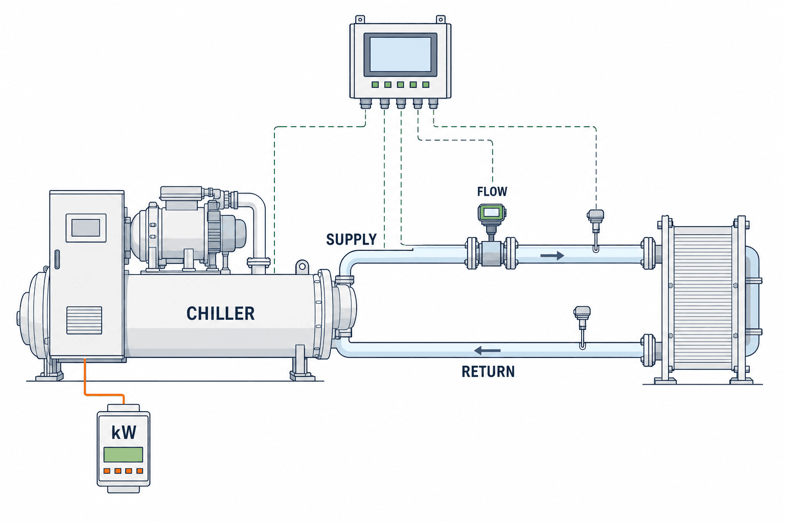
Figure 1 shows temperature, flow and power points between one chiller and a process heat exchanger. Check the actual plant’s pumps, shared headers, standby units, bypass routing and meter locations separately against the P&ID.
Calculate kW/ton with an explicit denominator
The cooling rate is the heat carried by the chilled water. For an illustrative water-based calculation:
Cooling rate (kW) ≈ 1.163 × flow (m³/h) × [return − supply temperature] (°C)
Cooling rate (RT) = cooling rate (kW) ÷ 3.517
kW/ton = electrical input (kW) within the same boundary ÷ cooling rate (RT)
The factor 1.163 approximates water density and specific heat. Correct the fluid properties when temperature or glycol concentration makes the water assumption unsuitable. RT is a U.S. refrigeration ton. DOE’s Energy Information Handbook illustrates monitoring a chilled-water system using flow, temperatures and electrical input [7]. For a header-level metric, use that header’s temperatures and flow, and the defined plant electrical input. For an individual chiller, pair evaporator-side measurements with that chiller’s power.
Take a hypothetical water flow of 60 m³/h, 7°C supply, 12°C return and 83 kW of power within a matching boundary. ΔT is 5°C. Cooling is 1.163 × 60 × 5 = 348.9 kW, or approximately 99.2 RT. The illustrative result is 0.84 kW/ton. If flow and input are artificially held constant but return falls to 10°C, ΔT becomes 3°C. Calculated cooling becomes 209.3 kW or about 59.5 RT, and the apparent ratio is about 1.39 kW/ton. This is an arithmetic example, not a diagnosis: real loads, compressor loading, pump operation and flow frequently change together.
| Illustrative assumption | Initial case | Lower-ΔT case |
|---|---|---|
| Flow | 60 m³/h | 60 m³/h |
| Supply / return | 7°C / 12°C | 7°C / 10°C |
| ΔT | 5°C | 3°C |
| Calculated cooling | 348.9 kW; about 99.2 RT | 209.3 kW; about 59.5 RT |
| Assumed same-boundary input | 83 kW | 83 kW |
| Calculated kW/ton | about 0.84 | about 1.39 |
When comparing with design, align cooling type, load fraction, ambient or condenser-water conditions, supply temperature, machine staging and meter scope. The water-cooled kW/ton figures in FEMP’s guide are conditional procurement benchmarks for U.S. federal buyers, not automatic pass/fail limits for a measured whole-plant figure in another facility [1]. Label COP or kW/kW separately if the dashboard provides those units.
Turn a low-ΔT alert into a diagnostic path
Low ΔT means the difference between chilled-water return and supply is smaller than the expected design or operating range. Look at it together with flow, load, valve positions, supply temperature and the number of machines running. Trane’s chilled-water clinic lists unbalanced flow, dirty filters or coils, air-handler controls and valve selection among common causes in HVAC systems [5]. In process cooling, also investigate heat-exchanger fouling, high flow after the process stops, open bypasses, three-way valves and unsuitable sensor placement.
First ask whether the measurement is credible. Two temperature probes with different calibration errors can substantially distort a small difference. A flow meter below its valid range, mismatched timestamps, inadequate resolution or a tag wired to the wrong sensor can do the same. Mark the calculated value invalid until the input problem is resolved. Then establish operating context: do not mix start-up, equipment changeover, cleaning recovery and production changeovers with stable-operation baselines. Compare periods with similar loads, staging and weather or condenser conditions.
An investigation can then check bypass and valve positions; differential pressure and pump speed; end-use inlet/outlet temperature; strainers, coils and heat exchangers; and finally instrument and control logic. Change the order to fit the site’s safe working procedure. Abruptly closing a bypass or reducing pump speed can violate a chiller’s minimum flow or a process’s cooling margin. Any control change should follow manufacturer limits, process requirements, responsible approval and a test plan. The Trane control overview is a starting point for plant-level thinking [4], not an instruction to alter a specific installation.

Figure 2 maps the chilled-water path, bypass and production heat exchanger for a low-ΔT investigation. An alarm should open a consistent sequence of checks, not automatically declare a failed component.
Separate process and HVAC requirements
For process cooling, define the protected product or machine temperature, acceptable excursion duration, response to lost cooling and how readings map to production batches or shifts. If demand tracks production, record line status, product changeovers and cleaning events beside the temperature trend. A failed standby pump can warrant an alarm even while the water temperature remains normal because redundancy has been lost. Use persistence times and actionable messages instead of instantaneous thresholds alone.
For HVAC chilled water, interpret readings alongside indoor conditions, outdoor air, air-handler operation, coil valve positions and occupancy. A single kW/ton threshold for both a lightly loaded night and peak daytime conditions can generate noise. Because low ΔT can originate at terminal units, inspect the load side before deciding to replace a chiller. ASHRAE’s controls design chapter covers the system context and equipment protection that a control design must consider [6]. It is not a substitute for a site’s own setpoints.
If one plant serves both production and HVAC, a common-header value alone will not express their different priorities. Identify branch meters or heat exchangers and put minimum process flow and temperature requirements ahead of optional optimization. Test the behavior during abnormal conditions before reallocating cooling capacity.
What to put in the URS and RFP
“Make the chiller visible through IoT” is too vague to test or price consistently. The user requirements specification (URS) should describe what operators need and how acceptance will be judged; the request for proposal (RFP) should let suppliers quote the same scope.
Purpose and scope. List target chillers and loops, process and HVAC uses, machine count, interfaces with the existing PLC/BMS, read-only monitoring versus permitted control commands, future expansion points, shutdown windows and permit constraints.
Measurement and computation. For each tag, give location, quantity, unit, instrument accuracy and range, communication method, sampling interval, time source, calibration and data owner. Specify the numerator and denominator for every kW/ton measure, handling of zero flow and stopped machines, fluid-property correction and aggregation period. One-minute raw data and a 15-minute aggregate are an example of a possible design choice, not a universal requirement; choose rates to match process dynamics and the network.
Display and use. On a plant schematic, show operating and communications state, CHWS, CHWR, ΔT, flow, cooling rate, power and kW/ton on a common time axis. Distinguish design values from measured values. Show “not calculable” when a machine is stopped or inputs are invalid. Allow users to trace a trend to the underlying tags and export data with role-based viewing and editing permissions.
Alarms. Define temperature excursions, rates of change, insufficient flow, link failure, open-circuit sensors, frozen values and mismatches between run status and power. For each alarm record severity, persistence, clear condition, recipient, out-of-hours escalation, suppression procedure and retention. Separate alarms that could affect product quality from instrument-maintenance alarms.
Data and connectivity. Do not replace missing readings with zero or present stale readings as current. Define reconnection and duplicate handling. Follow the site’s IT/OT policy for network segregation, authentication, logs, updates, storage and access. Make it practical for maintenance staff to reconcile the remote display against field instruments.
Deliverables and ownership. Require wiring and instrumentation diagrams, a tag dictionary, calculation specification, alarm matrix, calibration evidence, FAT/SAT records, operating guide and service contacts. State which party owns field meters, PLC work, gateways, storage and the dashboard, including interfaces to the existing equipment supplier.
Test the full chain at FAT and SAT
Factory acceptance testing (FAT) checks functions before delivery; site acceptance testing (SAT) verifies installed behavior. A FAT with simulated signals cannot establish that the temperature probe is in the intended pipe, a power meter has the correct CT ratio or a run signal is wired to the right machine. Record the source, expected result, tolerance, tester and evidence for each tag. Derive tolerances from the instrument specification and process requirement.
At FAT, simulate normal, high, low, disconnected, frozen, communications-lost, clock-skewed, stopped and restarted states. Compare cooling and kW/ton output with a hand calculation. Confirm that zero flow or missing inputs produce “not calculable.” Test alarm persistence, clearing, duplicate suppression and permissions. Match coefficients and rounding between the tag specification and display.
At SAT, compare field displays, PLC/BMS readings and monitoring values at the same time. Verify sensor location, flow direction, meter scaling and tag mapping during normal chiller and pump changeovers. Use safe simulated inputs and normal operating changes; do not deliberately put production outside safe temperature limits. Have the responsible operator receive an alarm and walk through the field response.

Figure 3 illustrates an alarm test: when the temperature-sensor connector is unplugged, the logger detects the lost sensor signal and the operator screen displays an alarm. Check any PLC/BMS and gateway in the real installation separately against drawings and field wiring.
Keep alarms and data quality usable
Distinguish an instrument problem from an equipment problem. If ΔT suddenly becomes zero, perhaps water temperatures converged; perhaps both tags read the same address. If a connection fails while the last value remains on screen, show its timestamp and stale status. Treating missing periods as zero energy makes a monthly report look improved for the wrong reason.
Give each tag a quality state such as valid, estimated, stale, missing or under calibration, and propagate it to calculations. Invalidate cooling and kW/ton when flow is outside the meter range. Record calibration deadlines and CT-ratio changes. Reassess the measurement boundary when a machine is replaced, even if a familiar tag name is reused. DOE’s Energy Information Handbook includes a chiller-plant monitoring example with plant kW/ton [7]; a useful dashboard also needs dependable data handling behind it.
Set thresholds using design conditions, stable historical operation and product requirements. A supply-temperature high alarm may call for immediate process-owner notification after an agreed persistence time. A sustained low-ΔT condition at similar load and valid flow may instead call for maintenance investigation. Review alarm counts, false positives and response time monthly, and keep a change log for threshold adjustments.
A practical implementation sequence
First collect P&IDs, electrical drawings, equipment records and existing trends. Reconcile real operating states and field readings with those documents; mark production and cleaning events. This baseline identifies missing instruments and data gaps. There is no need to promise savings at this stage.
Second, instrument one important loop. Align CHWS, CHWR, flow, matching power, equipment state and timestamps within one boundary. Review quality-marked trends with operators, verify calculations by hand and exercise notification during off-hours. Plan installation that requires a production stop with the production team.
Third, use comparable operating periods to investigate low ΔT, excess flow, cycling and setpoint deviations. DOE’s process-cooling cheat sheet lists variable-flow conversion and supply-temperature reset among possible measures [3]. Check chiller minimum flow, process temperature, warranty and control interactions before applying any of them. Monitoring finds a hypothesis; a field check verifies the cause; a controlled before/after comparison evaluates a change.
Finally, extend proven tag naming, test tables, alarm logic and display conventions to other loops, while redesigning boundaries for each air-cooled or water-cooled, process or HVAC application. If the plant also monitors towers, the cooling tower water-quality guide covers a related operating concern. The factory solar monitoring guide shares the principles of meter boundaries and data quality for another factory utility.
When comparing proposals, place meter installation and calibration, PLC/BMS changes, communications licences, storage, notifications, site tests, operator training and support on the same cost schedule. Confirm both first-year and recurring charges. Typical failures include temperature data without flow, power from a mismatched boundary, an unmanageable alarm flood, hidden communications gaps and a FAT that never leads to field verification. A precise tag list, calculation definition, alarm matrix and SAT record address these failures more directly than an additional dashboard panel.
Summary
A useful factory chiller monitoring system begins with the process or HVAC load to protect and a defined measurement boundary. Chilled-water supply and return temperatures, flow, matching power and machine state support a meaningful cooling-rate and kW/ton calculation. Investigate low ΔT through data quality, operating context, bypasses and end uses before assigning a fault. Put those definitions, alarms and FAT/SAT checks into the URS and RFP so that the finished system can be accepted and maintained.
TOMAS TECH can help map an existing plant, select measurement points, connect PLC/BMS data and define field acceptance tests around production needs. Share the chiller configuration, drawings and current problem through our contact page.
References
- U.S. Department of Energy, FEMP, Purchasing Energy-Efficient Electric Chillers — conditional air-/water-cooled and full-/part-load comparisons.
- U.S. Department of Energy, Improving Chilled Water System Performance — chilled-water system operation and assessment.
- U.S. Department of Energy, Better Plants, Process Cooling System Info Card — possible process-cooling improvements.
- Trane, Chiller Plant Control and Optimization — plant-level control overview.
- Trane, Air Conditioning Clinic: Chilled-Water Systems — low-ΔT causes and controls.
- ASHRAE, ASHRAE Handbook: Design and Application of Controls, Chapter 48 — control design context.
- U.S. Department of Energy, Energy Information Handbook — chiller-plant monitoring example.


