


What sets the electricity bill at a Thai factory is not how many kilowatt-hours you burned during the month. It is the single 15-minute interval in which you drew the most power. Manufacturers with Japanese parent companies arrive with a 30-minute average in their heads, because that is how high-voltage demand is measured in Japan, and they design demand control accordingly. In Thailand, the metering window used by MEA and PEA is 15 minutes. Half the window means half the room to dilute a spike. Run exactly the same operation with a Japanese-sized assumption and the meter can record 100 kW more. This article follows the numbers from the tariff definition all the way to payback.
What Demand Control Is: A 15-Minute Maximum Sets Your Demand Charge
Demand control means monitoring load, and shedding it when necessary, so that average demand over a defined interval does not exceed a set threshold. The objective is not to consume fewer units of electricity. It is to lower the single tallest peak that occurs once in the month.
This is exactly where demand control diverges from a conventional energy-saving program. LED retrofits, standby power reduction, and yield improvements that cut total production energy all reduce kilowatt-hours. They genuinely shrink the energy charge line on the invoice. But if the maximum demand in kilowatts does not change, the kW demand charge line does not fall by a single baht.
The reverse is also true: you can cut the demand charge without cutting output by a single unit. A compressor start, an electric furnace ramp, and the simultaneous restart of HVAC after lunch happened to land in the same 15 minutes. Stagger that overlap and production is unchanged while the peak drops. That is why demand control is treated as a separate discipline from energy saving.
Why 15 Minutes: How the Thai Tariff Defines It
What the demand charge is applied to in Thailand is the highest 15-minute average demand recorded during the billing month. The meter continuously records the average kW over each successive 15-minute interval, and at month end exactly one value, the maximum, is picked up. That one value is multiplied by a rate in THB/kW determined by your tariff type and supply voltage, and that product is your demand charge for the month.
Which tariff type applies depends on the size of your demand.
| Tariff | Scope | Treatment of demand charge |
|---|---|---|
| Type 3 (medium general service) | 30-999 kW | Demand charge applies. TOU is optional |
| Type 4 (large general service) | Maximum 15-minute average demand of 1,000 kW or more, or more than 250,000 kWh per month on a single meter | Demand charge applies. Choose TOU or TOD |
Mid-sized Japanese-affiliated plants typically fall under Type 3, while plants running moulding machines, furnaces, or large HVAC loads more often land in Type 4. Note also that Bangkok, Nonthaburi, and Samut Prakan are supplied by MEA, and every other province by PEA. The two utilities share the same tariff structure but publish separate rates, so the first thing to confirm is which table your own invoice is calculated from. The rates used throughout this article are MEA Type 4.
Two more items ride on the invoice: a service charge of 312.24 THB per month, and Ft, the fuel adjustment charge. For May to August 2026 the Ft is +0.1623 THB per unit. The point worth internalising is that Ft is an adjustment added per unit of energy consumed, and it does not apply to the kW demand charge. When Ft rises, what helps is reducing energy. What helps the demand charge is reducing the peak. Two measures with different targets should not be lumped together under one phrase such as “cutting the electricity bill.”
How This Differs from Japan’s 30-Minute Demand (100 kW on Identical Operations)
Production engineers transferred in from a Japanese parent company arrive, almost without exception, thinking in 30-minute demand. This is the first fault line.
| Point | Japan (high voltage) | Thailand (MEA/PEA Type 3 and 4) |
|---|---|---|
| Metering window | 30-minute average | 15-minute average |
| How the fixed charge is set | Contract demand equals the highest demand across the current month and the previous 11 months (actual-demand method, under 500 kW) | Monthly maximum 15-minute demand multiplied by the demand charge rate |
| Effect after a peak is recorded | Once recorded, it is carried for 12 months | Resets monthly, but 70% of the highest demand charge of the past 12 months acts as a floor |
| Consequence | Peaks are easily diluted, but heavy once recorded | Peaks are easily recorded as they are, but the after-effect is lighter |
The financial size of that difference is easiest to see in a single load event. Take a plant with a base load of 1,200 kW that runs a 300 kW piece of equipment for just 10 minutes.
- Value recorded in a 15-minute window = 1,200 + 300 x (10 / 15) = 1,400 kW
- Value recorded in a 30-minute window = 1,200 + 300 x (10 / 30) = 1,300 kW
The operation is identical. Same equipment, same run time, not one kWh of difference in energy consumed. Yet the recorded value differs by 100 kW. On Type 4 at 12-24 kV, those 100 kW are worth 13,293 THB per month (100 x 132.93).
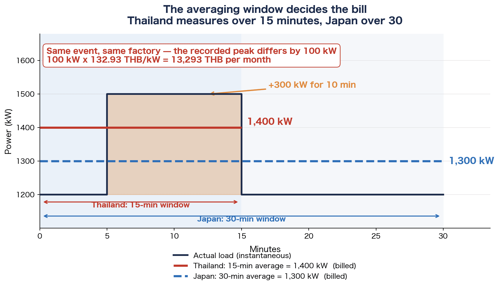
The reason is simple arithmetic: a 10-minute injection occupies two thirds of a 15-minute window but only one third of a 30-minute one. In Japan the width of the window acted as a denominator that automatically diluted short inrush events. In Thailand that denominator is halved.
Heavier in practice is that your reaction time is halved too. A Japanese-specification demand alarm predicts where the window will land, using elapsed time within the 30-minute window and accumulated energy so far, and raises an alarm if the landing point looks dangerous. Detect an anomaly in the first half of the window and you still had 15 minutes or more to shed load and pull the average back down. In a 15-minute window, the same “detected in the first half” leaves roughly 7 minutes. For someone to hear an alarm, walk to the equipment, confirm the situation, and operate a shutdown, that is clearly not enough.
Porting the setpoints and alarm logic of a demand controller straight from Japan is therefore risky. If you do bring it over, at least these three elements need to be rebuilt.
- Window synchronisation. Align the start time of the controller’s measurement window with the utility meter’s window. If they drift apart, the controller can show you inside the limit while the meter records a peak.
- Earlier alarms. Instead of relying on landing-point prediction, design a first-stage alarm that fires early on instantaneous value and rate of rise.
- Automatic shedding. Drop the assumption that a person can act within 7 minutes, and let the controller shed a pre-agreed list of loads by itself. This choice moves the cost picture significantly, so it is compared later in payback years.
How Factory Electricity Cost in Thailand Is Built (Type 3, Type 4, TOU and TOD)
A factory invoice is broadly made up of the demand charge (kW), the energy charge (kWh), the service charge, Ft, and the power factor charge. Of these, the demand charge generally accounts for 20-30% of the total billed amount.
Energy cost reduction in manufacturing tends to be discussed purely in kWh terms, and a team that only watches kWh can finish an entire programme without ever touching the 20-30% of the invoice that sits in the demand line. It is also the part with the most headroom to be reduced without capital expenditure. The wider picture of measurement architecture is covered in how to structure and select an energy monitoring system, but demand is one of the few indicators there where the money moves on the very first invoice after you start measuring.
The kW Demand Charge Rate Varies by a Factor of 2.83 with Supply Voltage
Same plant, same operation, same kW reduction, and yet the value of that reduction changes purely with your supply voltage. The MEA Type 4 TOU demand charge rates are as follows.
| Supply voltage | TOU demand charge (THB/kW-month) | TOD on-peak demand charge (THB/kW) |
|---|---|---|
| 69 kV and above | 74.14 | 224.30 |
| 12-24 kV | 132.93 | 285.05 |
| Below 12 kV | 210.00 | 332.71 |
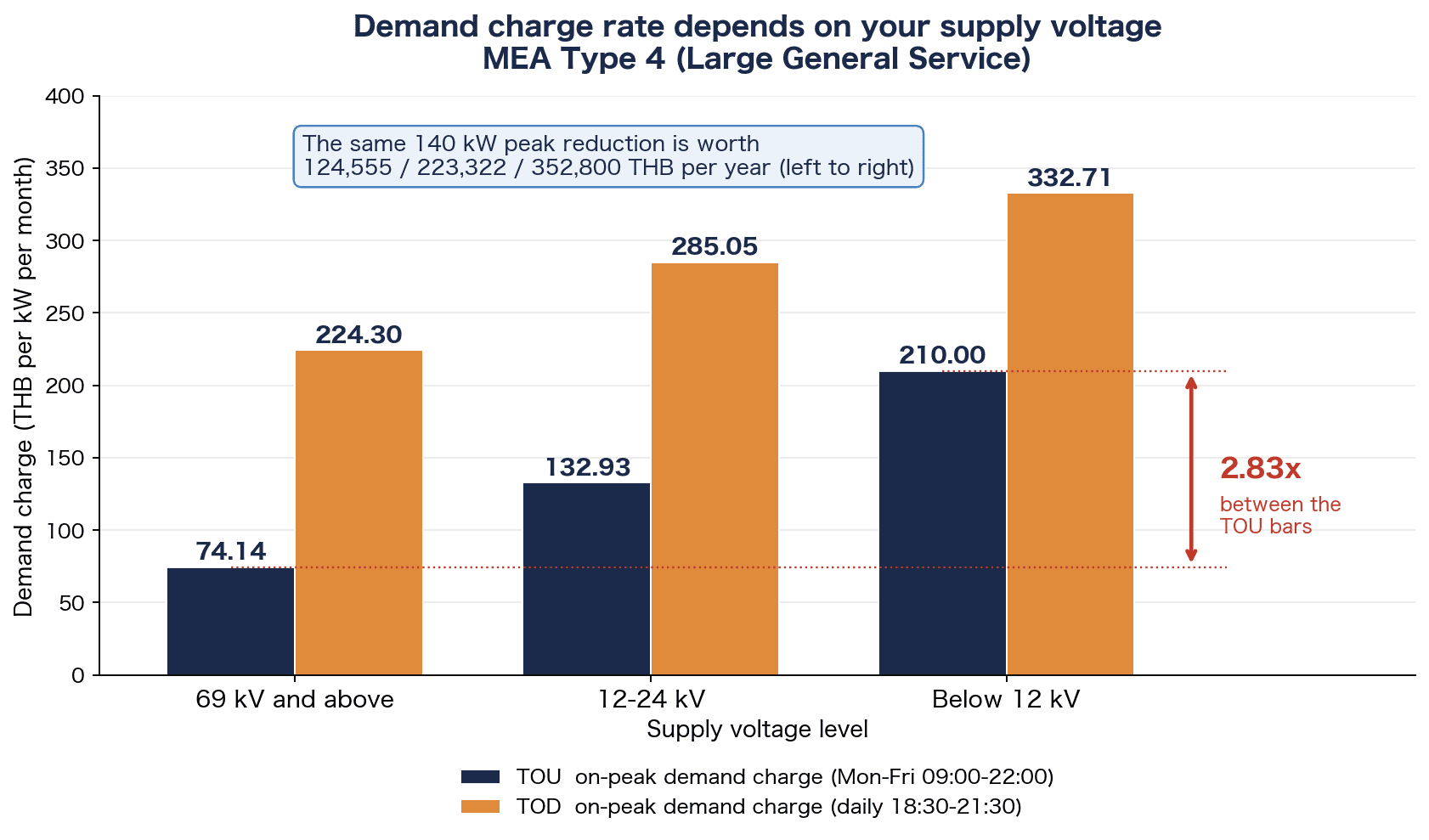
Here is the annual saving from a successful 140 kW peak reduction, laid out by voltage class.
| Supply voltage | Monthly saving | Annual saving |
|---|---|---|
| 69 kV and above | 140 x 74.14 | 124,555 THB |
| 12-24 kV | 140 x 132.93 | 223,322 THB |
| Below 12 kV | 140 x 210.00 | 352,800 THB |
The ratio between highest and lowest is 2.83 times (352,800 / 124,555). The very same 140 kW of peak demand reduction is worth 352,800 THB a year at a plant supplied below 12 kV, and only 124,555 THB a year at a plant supplied at 69 kV or above.
The decision rule that falls out of this is clear. Confirm your voltage class before you start evaluating demand monitoring or peak shaving investment. For the same capital outlay and the same kW reduction, payback at a sub-12 kV plant is close to a third of the payback at a 69 kV plant. Before taking someone else’s success story and concluding “we should get payback in two years as well,” ask what voltage that plant is supplied at. That question alone sharpens the estimate considerably.
The TOD on-peak demand rates look higher than the TOU rates, but as covered below they come packaged with an off-peak demand charge of zero. Rates cannot be judged cheap or expensive by lining up unit prices alone.
TOU or TOD: Which Is Cheaper Flips with Your Night-Shift Ratio
Under Type 4 you choose either TOU (Time of Use) or TOD (Time of Day). The two apply the demand charge in fundamentally different ways.
| Item | TOU | TOD |
|---|---|---|
| What the demand charge applies to | Maximum demand during on-peak (weekdays 09:00-22:00) | Maximum demand in each of on-peak (18:30-21:30), partial peak (daytime), and off-peak (late night) |
| On-peak demand charge (12-24 kV) | 132.93 THB/kW | 285.05 THB/kW |
| Partial peak demand charge (12-24 kV) | not applicable | 58.88 THB/kW |
| Off-peak demand charge | not charged | 0 |
| Energy charge | Separate rates for on-peak and off-peak | Separate rates by time band |
TOD on-peak at 12-24 kV is 285.05 THB/kW, more than double the TOU rate of 132.93 THB/kW. Under TOD, however, demand after 21:30 and in the early morning carries no charge at all because the off-peak demand charge is zero. Partial peak is also held low, at 58.88 THB/kW for 12-24 kV.
The choice therefore turns on one question: when does your peak occur?
- Day-shift plants where production has largely wound down between 18:30 and 21:30 can benefit from TOD. The daytime peak attracts only the cheaper partial peak rate (partial peak is charged only on the portion that exceeds the on-peak demand), and there is no peak during the expensive evening band.
- Plants that run continuously from evening into the night, or two- and three-shift plants with a high steady load at night, will inevitably create a peak in the evening band and take the TOD on-peak rate head on. TOU is more likely to work out cheaper.
- Night-oriented plants with a light daytime load get strong leverage from the zero TOD off-peak demand charge.
What this decision needs is data, not opinion. With one or two months of measured 15-minute demand broken down by time band, you can run both tariff tables and produce the answer as an amount of money. Put the other way round, a plant that has chosen TOU or TOD without measurement has chosen without evidence. Because switching contracts involves procedures and timing constraints, the sequence is: measure first, model second, apply third.
One further caution: choosing TOD changes the design of your operations themselves. With an off-peak demand charge of zero, there is a strong incentive to move heavy processes into the night. But unless night-shift labour cost, quality control coverage, and maintenance staffing move with it, what you gain on electricity you lose elsewhere. Do not reshape operations from the tariff table alone.
Do Not Overlook the Power Factor Charge
There is one more non-kW charge sitting on the same invoice: the power factor charge.
The rule is simple. Maximum 15-minute average lagging reactive demand (kVAR) in excess of 61.97% of the maximum 15-minute average active demand (kW) is charged at 56.07 THB per kVAR. Here too the basis is the highest 15-minute average. The figure 61.97% corresponds to a power factor of 0.85, since at 0.85 the ratio of reactive to active power is 0.6197. In substance, it is a charge that starts when your power factor falls below 0.85.
For a month with a maximum 15-minute average active demand of 1,400 kW, for example, the charge-free line is 1,400 x 0.6197 = 867.58 kVAR. Only the portion above that is billed at 56.07 THB/kVAR.
This line is easy to miss if you watch demand alone, and the reasons it gets missed are well understood.
- Capacitor banks degrade. Capacitors more than ten years old may have lost capacitance, and there is no guarantee that the power factor at commissioning still holds.
- It worsens at light load. As more equipment moves to inverter drives, power factor can drop in the low-load range. Plants with long periods of light-load running at night or at weekends deserve particular attention.
- It is not measured. Most plants read kWh, but few keep a continuous record of kVARh.
If you are installing a meter for demand monitoring anyway, the same instrument will give you kVAR and power factor. The additional cost is close to zero, and another line of the invoice becomes visible. For sensor and instrument selection, see also choosing IoT sensors for a factory.
The 70% Floor (Minimum Charge): Improvements Pay Fast, Accidents Linger 12 Months
The part of the Thai tariff that is structurally most unlike Japan is this floor.
The minimum charge in Thailand is defined as 70% of the highest demand charge of the past 12 months. However low your actual demand is in a given month, you will always be billed at least 70% of the demand charge from the most expensive month of the last year.
Under Japan’s actual-demand method (below 500 kW), the maximum across the previous 11 months and the current month becomes the contract demand outright, so a recorded peak is carried at 100% for 12 months. Thailand resets monthly and carries only 70%. That difference produces two asymmetric consequences.
A 10% Reduction Does Not Touch the Floor
Start with a model plant. Every number that follows comes from these assumptions.
| Item | Value |
|---|---|
| Supply voltage | 12-24 kV |
| Tariff | Type 4 / TOU |
| Monthly maximum demand | 1,400 kW |
| Demand charge rate | 132.93 THB/kW-month |
| Monthly demand charge | 1,400 x 132.93 = 186,102 THB |
| Annual demand charge | 2,233,224 THB |
Suppose this plant achieves a 10% peak reduction, that is 140 kW.
- Monthly saving = 140 x 132.93 = 18,610.2 THB
- Annual saving = 223,322 THB
- Demand after reduction = 1,260 kW
- The 70% floor = 1,400 x 0.7 = 980 kW
At 1,260 kW the plant sits above the 980 kW floor, so the floor is not reached. The full 140 kW of reduction flows straight through to a lower bill.
The floor only starts to bite once the reduction exceeds 30%. Thirty percent of 1,400 kW is 420 kW. Reduce by more than 420 kW and demand after reduction falls under the 980 kW floor, at which point further cuts stop lowering the bill.
The practical conclusion is this. At the 10-20% peak reduction most plants realistically target, the floor is not an obstacle. The improvement converts directly into money. And unlike Japan, nothing is dragged forward from last year’s record, so the effect appears in the month after the improvement. Anyone who has lived with “the contract demand you created once will not come down for 12 months” in Japan tends to be surprised by how quickly it lands here. Thailand is a system in which demand improvement pays off fast.
There are cases where the floor does deserve attention: a large solar installation, or moving a line to another plant, or anything else that makes demand fall structurally by more than 30%. In that situation the floor is active for the 12 months immediately after the drop, and the bill stays higher than the plant’s actual profile. Ignoring those 12 months in a payback model overstates the first-year benefit.
One 15-Minute Accidental Peak Costs 167,492 THB
The floor also works in the opposite direction. This is the main event.
Take a plant that normally runs steadily at 1,200 kW and, on one single occasion, records 1,800 kW for 15 minutes. Simultaneous equipment starts, a commissioning run, chillers all coming back together, or the start-up day of a new line. The cause does not matter. Here is what happens.
| Item | Calculation | Amount |
|---|---|---|
| Increment in the incident month | (1,800 – 1,200) x 132.93 | 79,758 THB |
| Resulting floor | 1,800 x 0.7 = 1,260 kW (above the normal 1,200 kW) | — |
| Increment over the remaining 11 months | (1,260 – 1,200) x 132.93 x 11 | 87,734 THB |
| Total | 79,758 + 87,734 | 167,492 THB |
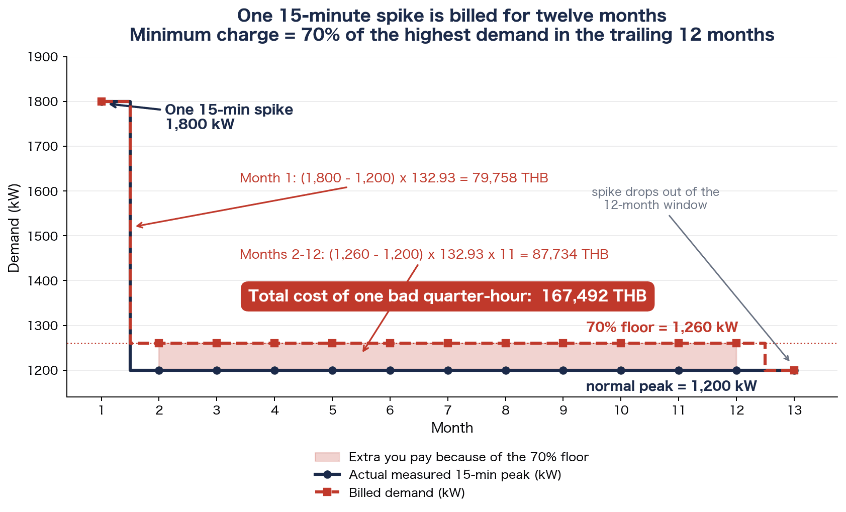
Fifteen minutes. A 15-minute lapse of judgement carries a price tag of 167,492 THB. What stings most is that the 87,734 THB spread over the following 11 months is larger than the 79,758 THB in the incident month itself. A plant that looks at the incident-month invoice, notes that it was a high month, and moves on will quietly pay roughly 7,976 THB every month for the next year (60 kW x 132.93 = 7,975.8 THB per month).
A 70% floor is a mercy in normal times. But build one tall peak and that 70% sits there for a year as a limit you cannot get under. It is lighter than Japan’s 100% carry-forward, which is not the same as light.
This structure feeds directly into the investment decision in the next section. The value of demand monitoring is not only in shaving a little off every month. It is in not letting this one event happen.
Demand Monitoring and Peak Shaving Costs Split into Three Layers
There is no single answer to “how much does a demand monitoring system cost,” because the order of magnitude depends on how far you go. In practice, thinking in three layers is what makes competing quotations comparable.
Layer 1 See, Layer 2 Separate, Layer 3 Stop
| Layer | What it does | Typical configuration | Cost range |
|---|---|---|---|
| Layer 1 See | Continuously monitor 15-minute demand at the incoming supply point and alarm on threshold breach | Pulse or Modbus pickup from the existing meter, one demand controller, alarm beacon | 120,000-250,000 THB |
| Layer 2 Separate | Identify which equipment is building the peak | CTs, power meters, and gateways on 10-20 main feeders | 400,000-900,000 THB |
| Layer 3 Stop | Automatically shed load as the threshold is approached | Automatic demand control of HVAC, compressors, chargers and similar, interlocks, PLC modification | Additional 300,000-800,000 THB |
The three layers have quite different characters.
Layer 1 is essential. A plant that cannot see its 15-minute demand at the supply point does not know when its own peaks occur. Considering energy investment before fixing that is like buying gym equipment without owning a scale. The cost is 120,000-250,000 THB, landing at the lower end if the existing meter already offers pulse output or Modbus communication, and at the upper end if the instrument itself has to be replaced.
Layer 2 is investment in root-cause identification. Watching the supply point alone tells you that this month was 1,400 kW again, but not what that 1,400 kW is made of. Only when consumption is measured per feeder do you reach a concrete fact such as “every Tuesday morning the furnace ramp coincides with two compressors starting.” Deciding which equipment to meter is also what determines the cost at this stage. The 400,000-900,000 THB range is set almost entirely by the number of measurement points (10-20), the difficulty of installing CTs, and whether a shutdown of the panel can be arranged.
Layer 3 is insurance. The next section puts numbers on that framing.
Payback: 2.69 Years Manual versus 3.58 Years Automatic, and Why You Still Choose Automatic
Using the model plant (12-24 kV, Type 4 TOU, 1,400 kW monthly maximum), here are two configurations compared on payback.
| Configuration | Capex | Annual running cost | Effective reduction | Annual saving | Net annual saving | Simple payback |
|---|---|---|---|---|---|---|
| Layer 1 only (see plus manual shedding) | 220,000 THB | 30,000 THB | 70 kW | 111,661 THB | 81,661 THB | 2.69 years |
| Layer 1 plus Layer 3 (see plus automatic shedding) | 620,000 THB | 50,000 THB | 140 kW | 223,322 THB | 173,322 THB | 3.58 years |
Effective reduction for Layer 1 is set at 70 kW because when a person has to act on the alarm, only half of what automation would shed is actually shed. Given that a 15-minute window leaves roughly 7 minutes between alarm and shutdown, that is not an optimistic assumption.
The result runs counter to most people’s intuition. On payback years, manual operation (2.69 years) beats automatic control (3.58 years). The reason is straightforward: automation adds 400,000 THB of capex (620,000 – 220,000) and 20,000 THB of annual running cost, while the reduction only doubles.
Looking at the increment alone makes it sharper still.
- Incremental net annual saving = 173,322 – 81,661 = 91,661 THB
- Incremental capex 400,000 THB / 91,661 THB = approximately 4.4 years
Isolate the additional 400,000 THB and it pays back in about 4.4 years. As a number for a capital request, that is weak. This is the point at which many plants conclude that they will put in Layer 1 first and see how it goes.
That conclusion is not wrong. But the comparison is being made on the wrong ground.
What the payback calculation contains is only the effect of shaving a little every month. The 167,492 THB cost of one accidental peak, from the previous section, appears nowhere in that table. Note also that the accidental-peak figure assumes a plant that normally runs at 1,200 kW, which is a different condition from the model plant above at 1,400 kW monthly maximum. Read it as an order of magnitude rather than adding it directly into the table. And an accidental peak, by definition, occurs when people could not respond in time. What Layer 1 manual operation can prevent is a foreseeable peak, not an unforeseen simultaneous start.
Consider a five-year evaluation period. If three accidental peaks occur over that period, the cost is 167,492 x 3 = 502,476 THB, which exceeds the 400,000 THB incremental capex for automation (around 500,000 THB if you include five years of the 20,000 THB per year incremental running cost). At two occurrences, it does not.
The decision therefore reduces to one question: how many unforeseen 15-minute peaks does our plant have in five years?
The material needed to answer that is precisely what Layer 1 gives you. Record 15-minute demand at the supply point for six to twelve months, and the number of times someone got there in time before the threshold was crossed, and the number of times it was crossed unnoticed, both emerge as actual data. A realistic sequence therefore looks like this.
- Install Layer 1 first and measure the frequency and causes of peaks (2.69-year payback, an investment that stands on its own)
- Use 6-12 months of measured data to establish the frequency of accidental peaks
- If the pace is three or more in five years, move to Layer 3. If it is below that, refine Layer 1 operations
Trying to justify automatic control on payback years will not get a capital request approved. Propose it as insurance. Whether the premium is reasonable is a question the Layer 1 data answers.
What to Shed First: Designing Load Priority
Install the hardware and, if nobody has decided what gets shed, all you have bought is an alarm. This is not a technical problem but a matter of agreement with the production department.
Loads You Can Shed and Loads You Must Not
The test is: when this load stops, what changes, and how long does it take to come back?
| Category | Examples | Judgement |
|---|---|---|
| Large thermal mass, state unchanged by a short stop | Office and canteen HVAC, warehouse HVAC, hot water | Can be shed. Room temperature barely moves over 15 minutes |
| Buffered, downstream not immediately affected | Compressors (where the receiver tank has headroom), some cooling water pumps, hot water storage | Can be shed conditionally. Pair with monitoring of buffer level |
| Shiftable in time | Forklift and AGV chargers, batch washing, test equipment, preheating of idle lines | Shed or shift. The safest place to find reduction |
| Quality changes if stopped | Constant-temperature chambers, plating baths, drying ovens, cleanroom HVAC | Do not shed |
| Long restart if stopped | Electric furnaces, extruder heaters, injection moulding barrels | Do not shed. Recovery cost exceeds the saving |
| Safety or regulatory | Exhaust fans, fire protection systems, ventilation in explosion-proof areas, emergency lighting | Never shed. Lock them out of scope with a hardware interlock |
Building this table is itself the core of the project. Exclude the never-shed loads from the scope with a hardware interlock at the design stage. Protect them with software setpoints alone and sooner or later somebody will edit a setting.
By far the easiest row to harvest reduction from is “shiftable in time.” Forklift chargers are numerous, each one draws a meaningful load, and shifting when they charge rarely disrupts operations. Despite that, many plants plug every truck in at once at the end of the shift. From a demand point of view that is the worst possible design. Simply staggering charge start times across the fleet lowers the peak at zero cost.
Compressors work well too, with one precondition. At a plant where air leaks have been left unaddressed, stopping a compressor drops pressure immediately and stops production. Leak repair is usually framed as an energy-saving measure, but from a demand control standpoint it is the enabling work that makes a compressor sheddable in the first place. See detecting and fixing compressed air leaks for the detail.
Operational Design on a Thai Site (Alarm Language, Shift Changes, Songkran and Chinese New Year)
Correct control logic does not lower the peak if operations do not work on the shop floor. Here are the points that specifically need designing at a plant in Thailand.
Alarm language and wording. A system that raises demand alarms only in Japanese, or only in English abbreviations, does not reach the people who actually operate the equipment. Issue alarms in Thai, and name the load to be shed. Not “demand exceedance alarm” but “please stop the HVAC in warehouse 2.” Not leaving the judgement to the operator is the condition for getting action inside the 7 minutes available.
Shift change windows. Around a handover, the outgoing shift’s equipment is still running while the incoming shift’s equipment starts up. Peaks form structurally, and attention is divided by the handover itself. A 15-minute window that straddles the changeover time is worth flagging as a watch period with its own monitoring settings.
The post-lunch restart. When HVAC and equipment come back simultaneously after the break, the peak concentrates in those 15 minutes. Staggering restart times by a few minutes per area costs nothing and works reliably.
Returning from long holidays. After Songkran in April, Chinese New Year, and the New Year break, idle equipment starts up all at once. Chillers, furnaces, and HVAC starting together produce a peak that normal operation would never generate. There is a paradox here: the accidental peak is most likely on the morning of the least productive day. Write the start-up sequence and the intervals between steps into the restart procedure. Unless it is written down, everything will be switched on at once.
Staff turnover. Do not let demand management depend on the instinct of one individual. Document the thresholds, the shedding order, and the contact list, and post them for each shift. Designing on the assumption that people change over faster than in Japan tends to produce something that lasts longer.
A 90-Day Roadmap for Rollout
Here is a standard 90-day sequence for making real progress on a limited budget.
| Period | What to do | Completion criteria |
|---|---|---|
| Days 1-15 | Analyse 12 months of invoices. Fix your tariff type (Type 3 or 4), TOU or TOD, supply voltage, monthly maximum demand, and whether a power factor charge applies | You have the highest demand of the past 12 months and the 70% floor calculated from it |
| Days 16-30 | Install Layer 1. Start recording 15-minute demand at the supply point. Check the output specification of the existing meter and replace the instrument if needed | 15-minute values are being recorded in sync with the utility meter’s window |
| Days 31-60 | Measure. Identify the day, time, and activity behind each peak. In parallel, build the load priority table (shed / do not shed) with the production department | The top three peak patterns are identified by the name of the equipment causing them |
| Days 61-75 | Execute the zero-cost measures. Stagger chargers, shift post-break restart times, formalise start-up sequences | The change in maximum demand before and after is confirmed numerically |
| Days 76-90 | Decide whether Layer 2 and Layer 3 are needed. Submit the capital request with the measured frequency of accidental peaks and a TOU / TOD switching model | You can explain it as “this happened this many times, so we are buying this much insurance” |
What matters in this order is that the zero-cost measures on days 61-75 are always executed first. If the numbers move there, the Layer 2 and Layer 3 request carries evidence that it actually worked at this plant. If they do not move, the cause identified in Layer 1 was wrong, and you have been spared from spending more.
The invoice analysis in days 1-15 can also be done in house rather than outsourced. The first two weeks cost nothing and carry the highest information content of the whole programme. Skip it and start collecting quotations, and you will be comparing prices without knowing what you are buying.
Frequently Asked Questions
What is demand control?
It is a mechanism that monitors electricity use and restricts load as needed so that average demand over a defined interval does not exceed a setpoint. In Thailand the monthly maximum of the 15-minute average is what the demand charge applies to, so the objective is to hold down the single tallest peak of the month. It differs from kWh reduction in both purpose and method, and it is possible to lower the demand charge without lowering output. The demand charge generally accounts for 20-30% of a factory’s billed amount.
How much does a demand monitoring system cost?
It splits into three layers by scope. Layer 1 (see), monitoring the supply point and raising alarms, runs 120,000-250,000 THB; Layer 2 (separate), metering 10-20 main feeders individually, runs 400,000-900,000 THB; and Layer 3 (stop), shedding load automatically as the threshold is approached, adds 300,000-800,000 THB. For a model plant supplied at 12-24 kV with a 1,400 kW monthly maximum, Layer 1 alone (220,000 THB capex, 30,000 THB annual running cost, 70 kW effective reduction) gives a simple payback of 2.69 years, and Layer 1 plus Layer 3 (620,000 THB capex, 50,000 THB annual running cost, 140 kW effective reduction) gives 3.58 years.
How do I reduce contract demand?
First, a premise: Thailand has no “contract demand carried for 12 months” equivalent to the Japanese actual-demand method. What is billed is the maximum 15-minute demand each month, and it resets monthly. Reduction is therefore achieved through operations that avoid creating a peak, not through a contract amendment procedure. Specifically: (1) measure 15-minute demand at the supply point, (2) identify the times and the equipment behind the peaks, (3) spread out shiftable loads such as chargers, batch processes, and preheating, and (4) decide which loads may be shed and drop them automatically or manually. Bear in mind, though, that 70% of the highest demand charge of the past 12 months remains as a floor, so for the 12 months immediately after a reduction greater than 30% the benefit is eroded by that floor.
What is the difference between peak shaving and peak shifting?
Peak shaving means stopping load during the peak period so that demand itself falls. Switching off HVAC or halting charging are examples. Peak shifting means moving demand to another time band rather than eliminating it, such as charging a battery at night and discharging it during the daytime peak, or running batch processes late at night. The end result for the demand charge is the same, but peak shaving sacrifices some production or comfort, while peak shifting requires either capital equipment or a change in operations. At plants on TOD, the zero off-peak demand charge makes peak shifting particularly valuable.
Expectations around peak shifting with a battery energy storage system (BESS) need care. Industrial LFP BESS, including PCS, BMS, and installation, runs roughly US$180-580/kWh globally, and in Thailand, with import and installation, tends to land in the upper half of that range. Straight arithmetic puts 2 MWh at US$360,000-1,160,000 (180-580 x 2,000 kWh). LFP cycle life is 4,000 to over 6,000 cycles, round-trip efficiency 85-90%, and service life 10-15 years.
The problem is on the revenue side. The industrial on-peak to off-peak energy price spread in Thailand is only about 1.5-1.7 THB/kWh (MEA Type 4 at 69 kV and above, TOU energy charge of 4.1025 on-peak and 2.5849 THB/kWh off-peak, a spread of 1.5176 THB/kWh). That spread alone will not pay back a battery. Only by stacking demand charge reduction, better use of surplus from existing solar, and backup value during outages does it become worth evaluating. Cases of 1 MW / 2 MWh paying back in 3.5 years do exist, but they are overseas cases built on a revenue stack of 40-50% peak shifting plus 20-30% frequency regulation, and they do not transfer directly to a typical plant in Thailand, because a Thai factory cannot be assumed to earn revenue from grid services such as frequency regulation. If you are evaluating a BESS, fix your own demand charge saving first (which, as shown above, varies by a factor of 2.83 with supply voltage), then stack the other values on top.
Will rooftop solar reduce my maximum demand?
It can, but there is no guarantee. There are three reasons.
First, demand is decided by one 15-minute interval per month. If a cloud passes over during that interval, output drops and demand does not come down. High annual generation and generating during that particular quarter hour are separate matters.
Second, the hours when your peak occurs and the hours when the array generates do not necessarily coincide. At plants that peak in the evening or at night, solar contributes almost nothing to the demand charge. For plants on TOD, on-peak is 18:30-21:30, when generation is essentially zero.
Third, there is the 70% floor described earlier. If solar drives demand structurally down by more than 30%, the floor is active for the following 12 months.
For that reason, booking demand charge reduction as certain income in a solar payback calculation is risky. Energy charge reduction can be booked, but demand reduction should be set conservatively, based on how far output falls on a poor generation day. Conversely, pair the array with storage so that discharge during the peak band is assured, and demand reduction becomes something you can treat as a planned figure. Reconciling measured generation against the invoice is covered in monitoring solar generation at a factory.
Summary
The points to hold on to for demand control at a plant in Thailand:
- The metering window is 15 minutes, not the 30 minutes used in Japan. Add 300 kW for 10 minutes on a 1,200 kW base and a 15-minute window records 1,400 kW while a 30-minute window records 1,300 kW. That is 100 kW on identical operations, worth 13,293 THB a month at 12-24 kV.
- Your reaction time is halved too. Japanese-specification landing-point prediction alarms do not act in time in a 15-minute window. Window synchronisation, earlier alarms, and automatic shedding all need rebuilding.
- The value of a reduction varies by a factor of 2.83 with supply voltage. The same 140 kW is worth 124,555 THB a year at 69 kV and above, 223,322 THB at 12-24 kV, and 352,800 THB below 12 kV. Confirm the voltage class before making the investment decision.
- TOU and TOD flip with your night-shift ratio. TOD on-peak (18:30-21:30) demand is expensive at 285.05 THB/kW for 12-24 kV, but off-peak is zero. Run measured data through both tables and compare in money.
- Power factor rides on the same invoice. Maximum 15-minute average lagging reactive demand above 61.97% of the maximum 15-minute average active demand (equivalent to a power factor of 0.85) is charged at 56.07 THB/kVAR. At 1,400 kW active, the charging line is 867.58 kVAR.
- The 70% floor does not obstruct improvement, but it does bite after an accident. A 1,400 kW plant cutting 10% (140 kW) stays above the 980 kW floor and banks the full 223,322 THB a year in savings. The floor only starts to bite beyond a 30% cut (more than 420 kW).
- One accidental peak costs 167,492 THB. A plant normally at 1,200 kW that creates 1,800 kW once for 15 minutes pays 79,758 THB in the incident month and 87,734 THB over the following 11 months. The after-effect is the larger part.
- Automatic control loses on payback years. Layer 1 alone is 2.69 years against 3.58 years for Layer 1 plus Layer 3, and about 4.4 years on the increment alone. Propose automation as insurance. The evidence for that decision is the frequency of accidental peaks, obtained by running Layer 1 for 6 to 12 months.
The first thing to do is not to invest. It is to lay out 12 months of invoices and fix your tariff type, supply voltage, monthly maximum demand, and whether a power factor charge applies. Those two weeks of work cost nothing and become the premise for every decision that follows.
When looking at demand control, it is not unusual to be unable to settle questions such as which tariff table your invoice is actually calculated from, whether the investment makes sense given your supply voltage, or whether TOU or TOD suits your operating pattern. TOMAS TECH supports the whole path, from a fact-based review built on your invoices and operating patterns through Layer 1 measurement to Layer 3 automatic control. We are happy to talk even if you are still at the evaluation stage and have not decided on anything. Feel free to get in touch through our contact page.
References
- MEA, “ประเภทที่ 4 กิจการขนาดใหญ่” (Type 4: Large General Service)
- PEA, “Latest Ft”
- BOI, “Utility Costs”
- EGAT, “อัตราค่าไฟฟ้า” (Electricity Tariff)
- CapSolar, “What Is Demand Charge?”
- CapSolar, “Thailand Electricity Price 2026”
- CapSolar, “Factory BESS TOU Arbitrage Payback (Thailand 2026)”
- J-Net21, “The relationship between contract demand and 30-minute demand values” (Japanese)
- Kansai Electric Power, “What is contract demand?” (Japanese)