



Three months after handing the inspection data to an AI vendor, the report came back saying that the defect rate was higher on Monday mornings. That was not what the plant manager wanted to know. He wanted to know what the holding pressure had been, in MPa, on the lot that came out with sink marks. AI analysis of quality inspection data cannot answer that question, and the reason is not a weak model or a small training set. It is that the unit in which defects occur and the unit in which manufacturing conditions are recorded are different. This article measures that gap with a metric called the matchable rate, and puts numbers on cost and payback using a plastic injection molding plant in Thailand as the model. The conclusion first: the scope that captures the finest data is not the scope that pays back fastest.
The real reason AI analysis of quality inspection data misses
“We have three years of quality data stored. Can we run AI analysis on it?” That question comes to us regularly from Japanese-owned plants in Thailand. The honest answer depends entirely on what is inside that data. And when we actually look inside, the answer is usually no. Not because there is too little data. Because what has been stored is not shaped in a way that can explain causes.
Training on inspection results alone will not surface causes
What most plants call “quality data” turns out to be a tally of inspection results. In terms of columns: date, shift, machine number, part number, defect category, defect count. Even in well-run plants, the most you tend to find on top of that is the inspector’s name and a time band.
So what happens when you hand that whole table to an AI? The algorithm looks through the columns it was given and searches for the ones that correlate with defect count. The only usable columns are date, shift, machine number and part number. So the answers that come back are combinations of those four. More defects on Monday mornings. More on machine 3. More on part number X. Each of those may well be true, but this is not analysis. It is aggregation, and a pivot table in Excel will produce it in five minutes.
Why does it end up this way? Because cause analysis is the work of searching for the variables that explain an outcome. If the explanatory variables are not in the data, no model of any kind will produce an explanation. Sink marks in injection molding come from holding pressure, cooling time, melt temperature and mold temperature, yet none of those columns exist in the table. What does not exist cannot be learned.
This is a failure the industry repeats. Gartner puts the share of AI projects that fail to achieve their original objectives at 70 to 85 percent (source). And the root of that failure is described as lying not in the performance of the AI itself, but in the poor quality of the input data. In Japanese manufacturing, the share of companies making use of digital technology rose from just under half in 2019 to more than 80 percent in 2023, while adoption remains low among companies with 300 employees or fewer, leaving a pronounced gap by company size (source). The model plant in this article has 320 employees, which puts it right on that boundary.
It is worth looking at the other side as well, at a case that worked. In one reported example, three years of past inspection data were used to train an AI, the insight that “this combination of temperature, humidity and processing speed raises the defect rate” was extracted and fed back to the production line, and the product defect rate was reduced by 30 percent. In the same case, the time to produce an inspection report fell from 30 minutes to 5 minutes, an 83 percent reduction (source).
The number to pay attention to in that case is not the 30 percent. It is that the training data contained temperature, humidity and processing speed as explanatory variables, in a form that could be lined up against the inspection results. The order of events is the reverse of what people assume. It was not that causes appeared because AI was introduced. It was that AI could do its job because variables capable of being causes were already aligned on the same axis. Note also that this 30 percent comes from another company’s case, and it is a different thing from the 25 percent reduction assumed in the model calculation later in this article. Please do not mix the two.
It is worth drawing a line here between this topic and the neighboring ones. AI in manufacturing can be organized by process into quality inspection (AI visual inspection and anomaly detection), equipment maintenance (predictive maintenance), and procurement and inventory (demand forecasting and inventory optimization) (source). Of these, finding defects from images is covered in our guide to introducing AI visual inspection. This article picks up where that one leaves off. It is about pinning down the cause of a defect that has already been found, using numerical data. A camera can tell you that a part is defective. It cannot tell you why it became defective.
The unit of a defect and the unit of a process condition do not line up
Put two shop-floor records side by side.
The first is the inspection record. “August 12, machine 3, sink marks, 12 pieces.” The second is the molding condition sheet. “August 12, shift A, machine 3, holding pressure 45 MPa, melt temperature 240°C, cooling 18 seconds.” It is handwritten, filled in once per shift by the line leader.
What can you say by matching those two? “During shift A, at a holding pressure of 45 MPa, 12 sink mark defects occurred.” That is all. You do not know at which moment within shift A those 12 pieces came out. And you do not actually know whether the holding pressure really stayed at 45 MPa for the full eight hours either, because what was recorded is a single value taken at the one moment the line leader walked over to look.
Let us fix the scale with the assumptions of the model plant. Twenty molding machines, 4-cavity molds, a 30-second cycle time, two shifts of 16 hours, 24 working days per month. That is 7,680 parts per machine per day, 153,600 per day across the plant, 3,686,400 per month and 44,236,800 per year. At a defect rate of 1.5 percent, annual defects come to 663,552 parts. Putting the loss per defective part at 2.50 THB for material and processing cost, the annual defect loss is 1,658,880.00 THB.
Every one of those 663,552 parts has a moment at which it was molded. With a 4-cavity mold, four parts come out simultaneously in a single shot. Sink marks and dimensional deviations alike occur within that shot. In other words, the unit in which defects occur is the shot. But the unit in which conditions are recorded is the shift. One is 30 seconds, the other is eight hours. Asking someone to match those two is close to asking them to read the time by laying a calendar over a clock that has only a second hand.
And this is not a “not enough data” problem. It is a different unit problem. Accumulate three years in the same plant, or ten years, and if the units differ the two sides still will not join up. Effort spent in the direction of increasing data volume does not get rewarded here.
Matchable rate: the metric to measure before accuracy
So where do you start? Not with precision, not with recall. You start by measuring the matchable rate.
What the matchable rate is and how to count it
The matchable rate is the proportion of defects for which you can uniquely link what was happening at the time the defect occurred. The denominator is the number of defects. The numerator is the number of those defects that are uniquely tied to condition data.
Counting it is simple, and it needs no system. Pull 50 recent defects from the log. Then, one by one, fill in yes or no against four questions. First, is the time of occurrence known to the minute, and preferably to the second? Second, can the molding conditions at that time be identified? Third, is it known which machine, which mold and which shot it came from? Fourth, is the material lot and the drying batch that was being fed at the time known?
The most important part here is the word “uniquely.” Anything filled in by inference counts as a no. “It must have been machine 3, because that is where we were running that part number that day” is a no. “The average conditions on shift A are roughly this” is also a no. A field that a human filled in from memory and instinct cannot be handed to a machine. Hand it over and it becomes training data with the wrong label attached.
Why measure this before accuracy? There are two reasons. The first is that defects that cannot be matched never enter the training data at all. If the matchable rate is 12 percent, then only a small fraction of the 663,552 defects can be used for cause analysis. However good the model is, it can say nothing about the part it cannot see.
The second reason is the more serious one. Data that has been forced into a linkage it does not actually support goes wrong in a way that does not announce itself as wrong. Even when the model returns a high accuracy figure, that figure may be an accuracy computed on top of a misaligned linkage. Accuracy is a metric that presupposes the matching is correct. Without measuring the foundation, you end up discussing the quality of the roof.
A four-stage model (current state, A, B, C)
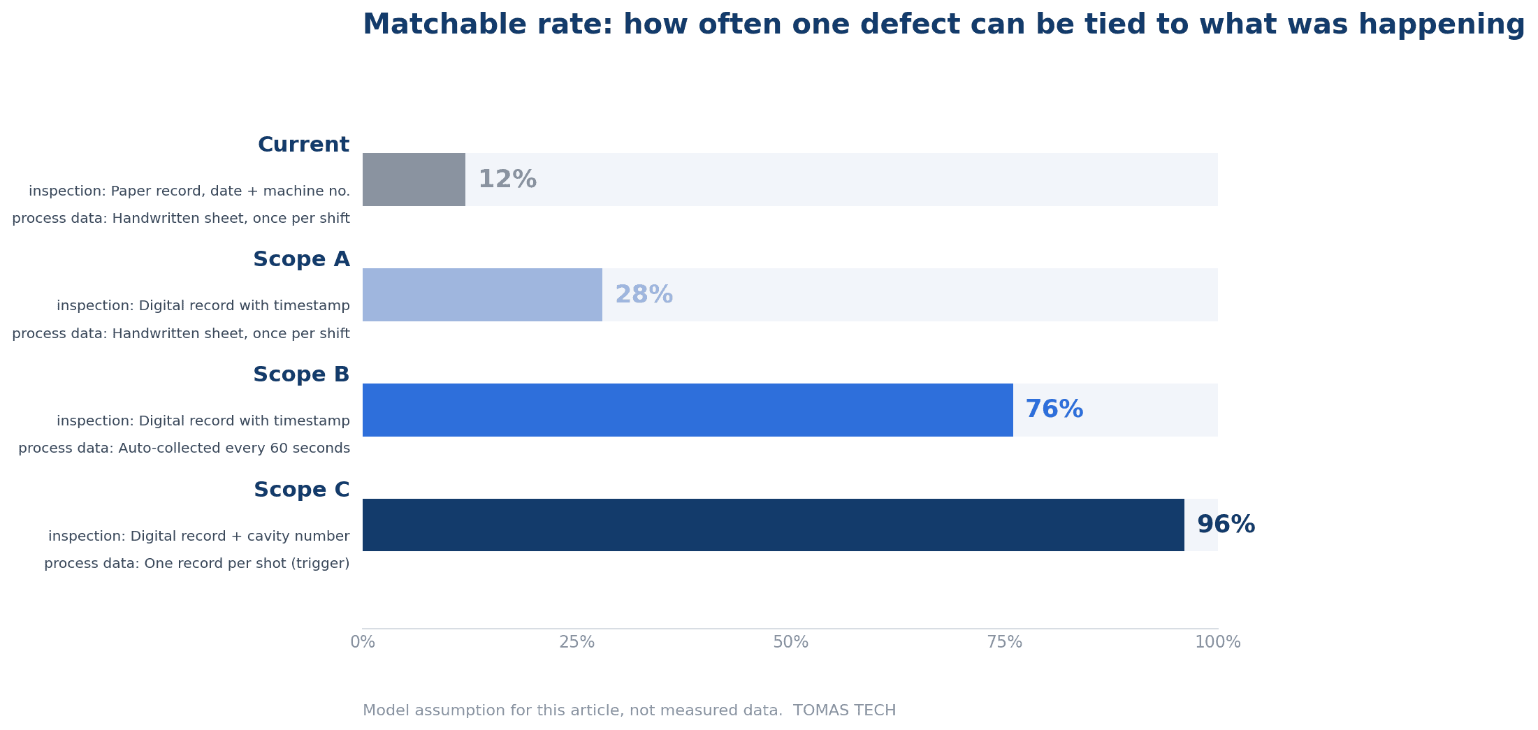
The table below models how the matchable rate changes at each stage of investment. These figures are the modeling assumptions of this article, not measured values from any specific plant. The shape of the progression, however, is common to many molding plants.
| Stage | Unit of the inspection record | Unit of the condition data | Matchable rate |
|---|---|---|---|
| Current state | Paper, date plus machine number | Handwritten condition sheet, once per shift | 12% |
| A | Electronic, per-part record with timestamp | Handwritten condition sheet, once per shift | 28% |
| B | Electronic, per-part record with timestamp | Automatic collection at 1-minute intervals | 76% |
| C | Per part plus cavity number | Per shot (trigger-based collection) | 96% |
The 12 percent in the current state covers the cases you can trace by luck even when conditions are coarse. The time of a material lot changeover happened to be written in the daily report, or a batch of defects appeared right after a mold change. Turn that around and it means the overwhelming majority of defects are being counted as defects with no record of what was happening at the time.
The stage to pay attention to is A. Even if you digitize the inspection record and give every single part a timestamp, you only reach 28 percent. The denominator is still all defects, and the condition side is still a handwritten sheet filled in once per shift. Tidying up only the inspection side does not produce a match if the counterpart you are matching against is coarse. This is the structural reason why projects that “handed the inspection data to a vendor” stall.
At B it jumps to 76 percent. Conditions are collected automatically from the molding machines at 1-minute intervals and placed on the same time axis as the inspection records. Only at this point do material-lot-related, drying-related and conveying-related defects become traceable. At C it reaches 96 percent. Trigger-based collection per shot and cavity numbers come in, and variation within a shot and differences between cavities become visible.
If the sampling interval is coarse, shot-level causes never appear
When we suggest to a plant that has stopped at A that it should start collecting conditions automatically, the next thing that always happens is a debate about the sampling interval. If that debate is settled casually with “a 1-minute interval should be fine,” it creates a gap that cannot be recovered later.
What disappears at a 1-minute interval on a 30-second cycle
The model plant runs a 30-second cycle time. That is 120 shots per machine per hour. Apply 1-minute collection to that and you capture a value only once every two shots. For the other half of the shots, what the temperature was and what the pressure was will not exist, permanently.
This is not a matter of accuracy being halved. It is a matter of shot-level tracing being impossible in principle. Sink marks and short shots do not necessarily appear in a continuous run. Material bridging or variation in the metering can push a single isolated shot out of condition. On an interval that does not record that one deviating shot, the fact of the deviation itself does not exist. Improving the model afterwards cannot restore data that was never there.
There is another trap in interval-based collection that is easy to overlook. It arises when the collection unit is configured to record “the average over that one minute.” Take an average and isolated outliers are always smoothed away. A peak in melt temperature, a dip in holding pressure, both vanish into the mean. Averaging is an operation for erasing anomalies, so holding data intended for anomaly detection or defect cause analysis as averages puts the means and the ends the wrong way round.
If you want to trace at the shot level, use trigger-based collection rather than interval-based collection. That means writing one record on receipt of the shot completion signal. One row per shot, so nothing is dropped. It requires taking a signal out of the equipment and configuring the PLC side, so for how to do that in practice, see our article on PLC data collection in practice.
That said, you do not need to put every machine and every item on trigger-based collection. As the next chapter shows, the defect modes that require shot-level data are limited. That becomes the central question of the second half of this article.
Before you raise the sampling rate, synchronize the clocks
There is a problem that should be settled before the debate about intervals. The clocks.
A plant contains any number of devices that hold a time. The input terminal in the inspection process, the molding machine controller, the data collection unit, the MES server, the PC in the office. Left alone, these clocks will always drift apart. On a device with no time synchronization configured, the internal clock accumulates drift little by little.
What happens on a line with a 30-second cycle time if the inspection terminal and the molding machine are two minutes apart? For a part recorded in inspection as “defect detected at 10:15,” the molding conditions that get linked to it are the values from two minutes earlier. With a 30-second cycle, many shots have gone past within those two minutes. You end up training the model on the conditions of a completely different shot as the cause of that defect.
The awkward part is that this error does not surface as an error. The data is complete, the row counts match, the model runs. Accuracy figures come out. It is just that all of the contents are shifted. And when the analysis results fail to match what the shop floor knows to be true, the thing that gets suspected is usually the model, not the clock. This is the cheapest available route to the conclusion that “AI is unreliable.”
So how closely do the clocks need to agree? This article uses one tenth of the cycle time, that is, within 3 seconds, as a working target. This is a value adopted here as a practical rule of thumb, not a value laid down in any standard. If you want a rationale for 3 seconds, the thinking is that it should be comfortably smaller than the duration of one shot. The idea is simply that it should stay within a range where you cannot mistake one shot for another.
In implementation terms, the basic approach is to stand up one NTP server inside the plant and synchronize terminals, collection units and servers to it. There are cases where the molding machine controller is old and does not support NTP. In that case, the practical route is to design the collection unit to apply the timestamp, and to decide outright that the controller’s clock will not be used for matching. Deciding on a single authority for time is safer than forcing a device that cannot synchronize into the chain. It also helps to keep a daily log recording the amount of drift, so that later you can judge that “the data from this period cannot be trusted.” On how to capture time on the inspection side, our article on designing automated inspection data collection is also a useful reference.
Different defect modes need different granularity: how fine is fine enough
Reading this far, you may be thinking that the answer is simply to capture everything at shot level and cavity level. Technically, that is correct. As an investment, it is not necessarily correct. The reason is that the unit in which a cause arises differs by defect mode.
| Defect mode | Unit in which it occurs | Granularity of condition data required | Scope that reaches it |
|---|---|---|---|
| Black spots and contamination (material-related) | Material lot | Material lot × time of charging | B |
| Silver streaks (insufficient drying) | Drying batch | Dryer batch × time | B |
| Ejection and conveying scratches | Individual part | Time × process step | B |
| Sink marks and short shots (condition variation) | Shot | Holding pressure and melt temperature per shot | C |
| Dimensional deviation (cavity-to-cavity difference) | Cavity | Cavity number | C |
Defects where material lot granularity is enough
The top three rows are modes where the unit in which the cause arises is coarser than a shot.
Take black spots and contamination. Where the cause lies on the material side, the cause is that something was mixed into that lot. A material lot is a unit of one bag or one pallet, and it takes hours to consume. So what you need is the material lot number and the time at which it was charged. With those two, you can trace it in the form of “after lot X was charged at 10:40, black spots increased.” Melt temperature per shot adds nothing to that judgment.
Silver streaks have the same structure. When insufficient drying is suspected, the unit is the dryer batch. It is enough to know which batch was used and when. Drying time and temperature per batch, plus the time of charging. These are captured perfectly well by 1-minute interval collection.
Ejection and conveying scratches are slightly different in character, in that the unit of occurrence is the individual part. But the condition data required is “time × process step,” not molding conditions per shot. To see whether the rubbing is happening at the take-out robot arm, on the conveyor or at the boxing process, it is enough to know when each part passed through which process step. This too works within the range of B.
What these three modes have in common is that the cause persists over a long period of time. A cause that persists can be caught even with a coarse record.
Defects that require shot-level and cavity-level data
The bottom two rows are different.
Sink marks and short shots, where the cause is condition variation, occur at shot level. Variation in metering, wear on the non-return ring, a poor bite on the material. These occur on one specific shot and return to normal on the next. As described in the previous chapter, a record taken once every two shots will not catch them. Only when trigger-based collection gives you one record per shot does the holding pressure and melt temperature of that one shot become visible.
Cavity-to-cavity dimensional deviation is more troublesome still. Suppose that in a 4-cavity mold, one cavity has a partially blocked cooling channel, or its venting has degraded. Only the parts coming out of that cavity deviate dimensionally. But if the inspection record has no cavity number, all four are seen as one group. Even when a single cavity is far out of tolerance, viewed as a distribution of four it looks like nothing more than “the variation is a little wide.” The cause is concentrated at one point, yet it is transformed into a problem of overall variation.
That transformation sends the countermeasure in fundamentally the wrong direction. Diagnosed as a variation problem, you end up touching the molding conditions as a whole. What was actually needed was cleaning the water channel of one cavity. The absence of a single column called cavity number is enough to make the correct countermeasure permanently unreachable. That is the reason Scope C exists.
Capturing cavity numbers requires engraving marks in the mold and a mechanism in the inspection process to read them. It is a modification to the mold, and it also adds work to inspection. It is not something a software configuration change can deliver.
Cost rises non-linearly as granularity rises
By this point it is clear that raising the granularity increases what you can see. The problem is that the way cost increases does not have the same shape as the way benefit increases.
Moving from B to C, what you additionally need is cavity identification (mold engraving and reading) at 22,000 THB per mold across 20 molds, plus model building and operational design at 200,000 THB. Initial cost rises from 1,660,000 THB to 2,300,000 THB. Annual cost also rises from 300,000 THB to 450,000 THB.
It is not only the money that increases. First, data volume. Trigger-based collection means one record per shot, so one machine produces 120 shots’ worth of rows per hour. That accumulates across 20 machines, two shifts of 16 hours, and 24 working days. Row counts jump compared with interval collection, and the storage and query design has to be reworked.
Second, operational load. Mold engraving means one more item falls under mold maintenance. If the engraving wears down it becomes unreadable, and an unreadable record becomes unmatchable. In the inspection process, the work of reading a cavity number on every part is added. Even at a few seconds per part, that is not negligible as a burden on inspectors.
Third, model operation. Shot-level data contains more outliers than coarse data. Immediately before and after equipment stoppages, ramp-up after a mold change, the transition period at a material changeover. Rules for excluding these have to be created and then maintained. This is not a task you do once at introduction and finish. It needs reviewing every time conditions change.
In other words, investing in C means buying not only the additional initial cost but also a permanent increase in operational weight. Whether your plant has defect modes that justify that weight is where the decision turns.

A model calculation for a Thai plant: assumptions and how the benefits are allocated
Let us put it into numbers. The assumptions for the model plant are as follows.
| Item | Value |
|---|---|
| Model plant | Thailand, plastic injection molding (tier 2 supplier of automotive interior parts), 320 employees |
| Molding machines | 20 machines, 4-cavity molds, 30-second cycle time |
| Operation | Two shifts of 16 hours, 24 working days per month |
| Output | 7,680 parts per machine per day, then 153,600 per day, then 3,686,400 per month, then 44,236,800 per year |
| Hourly rate, quality and molding engineers | Monthly salary 45,000 THB × factor 1.2 ÷ 160h = 337.5 THB/h |
| Hourly rate, administrative staff | Monthly salary 28,000 THB × factor 1.2 ÷ 160h = 210.0 THB/h |
| Defect rate (current) | 1.5%, giving 663,552 defective parts per year |
| Loss per defective part | 2.50 THB/part, giving an annual defect loss of 1,658,880.00 THB |
| Assumed defect reduction | 25% reduction (equal to 165,888 parts) |
A note on the hourly rate assumptions. Wages in Thailand are on an upward trend, and the wage increase rate at Japanese-owned companies was 3.8 percent in 2023, 4.58 percent in 2024, and is projected at 4.64 percent for 2025. The minimum wage was also revised on January 1, 2025 to a daily rate of 337 to 400 THB, with Bangkok at 372 THB (source, source). This article calculates at current hourly rates without building in those increases, but benefits of the labor-saving type tend to grow in monetary terms year by year. In that sense the estimates below take a conservative view of the benefit side.
Four benefit streams are set out.
| # | Benefit | Calculation | Amount (THB/year) |
|---|---|---|---|
| 1 | Defect reduction | 663,552 parts × 25% = 165,888 parts × 2.50 | 414,720.00 |
| 2 | Labor for cause analysis | 48 cases/year × (40h – 16h) = 1,152h × 337.5 | 388,800.00 |
| 3 | Labor for matching inspection records against condition sheets | 2 shifts × 1 person × 1.5h × 24 days × 12 months = 864h × 80% = 691.2h × 210.0 | 145,152.00 |
| 4 | Condition setup after mold changes | 480 changes/year × 0.6h = 288h × 337.5 | 97,200.00 |
| Total (Scope C) | 1,045,872.00 |
Benefit 1 assumes a 25 percent reduction of the 663,552 annual defects. This 25 percent is a modeling assumption of this article, not an actual result. It is a different figure from the 30 percent reduction in the other company’s case introduced earlier, so please do not mix them. The 165,888 parts eliminated are multiplied by the loss of 2.50 THB per part to give 414,720.00 THB.
Benefit 2 is the labor for the cause analysis that gets triggered every time defects appear. The assumption is 48 cases per year, that is, four analysis cases per month. The setup is that a case which used to take 40 hours takes 16 hours. Most of those 40 hours consists of gathering paperwork, transcribing condition sheets, and building charts in Excel, with very little of it actually spent thinking. When matched data is already at hand, that front end disappears. At 1,152 hours per year and an engineer rate of 337.5 THB, that is 388,800.00 THB.
Benefit 3 is the day-to-day matching. On each of the two shifts, one person spends 1.5 hours a day matching inspection records against molding condition sheets and compiling the daily report. Across 24 days and 12 months that is 864 hours per year. An 80 percent reduction saves 691.2 hours, and that saving at the administrative rate of 210.0 THB comes to 145,152.00 THB. This work differs in character from the other three in that it occurs every day whether defects appear or not.
Benefit 4 is condition setup after a mold change. The assumption is that for each of 480 mold changes per year, the adjustment time until good parts come out consistently is shortened by 0.6 hours. If the conditions from a previous run of good parts with the same mold and the same material can be retrieved with timestamps attached, those can be used as the starting values. At 288 hours per year and 337.5 THB, that is 97,200.00 THB.
A word on the investment environment as well. Investment applications in Thailand in the first half of 2026 reached USD 43.6 billion across 1,299 projects, up 37 percent year on year, of which the digital sector accounted for USD 33 billion (source). Under the BOI’s “Smart and Sustainable Industry” measures, 132 applications worth USD 507.6 million were submitted for machinery upgrades, digital technology adoption and automation robot integration (source). Whether such schemes apply is decided case by case, so they are not built into the estimates below. When you put this in front of an approval committee, check separately whether your own company qualifies.
The allocation of benefits also needs its assumptions stated. How are the four benefit streams above distributed across Scopes A, B and C? This article sets them out as follows.
- A = benefit 3 (145,152.00) + 30% of benefit 2 (116,640.00) = 261,792.00
- B = A + the remaining 70% of benefit 2 (272,160.00) + benefit 4 (97,200.00) + 60% of benefit 1 (248,832.00) = 879,984.00
- C = B + the remaining 40% of benefit 1 (165,888.00) = 1,045,872.00
Benefit 1 is split 6 to 4 between B and C because, in the defect mode table in the previous chapter, the modes reachable by B (black spots and contamination, silver streaks, conveying scratches) are assumed to account for 60 percent on a monetary basis. That 60 percent is an assumption of this article, not a measured value. If the breakdown of your own defect pie is different, this allocation changes. And as discussed below, this ratio is precisely what the conclusion turns on.
Cost and payback: the scope that hits hardest is not the fastest to pay back
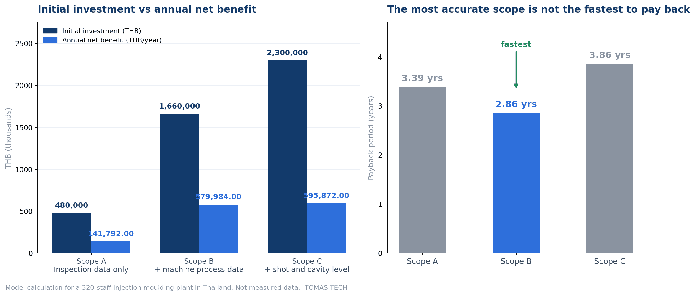
Let us compare the three scopes. In terms of matchable rate, A is 28 percent, B is 76 percent and C is 96 percent. The degree to which the analysis hits its target is highest at C. Does that mean payback is fastest there too? It does not.
Scope A: AI analysis on inspection data alone (3.39 years)
Digitizing the inspection records costs 300,000 THB (eight terminals and form design), and a BI visualization platform costs 180,000 THB. Initial cost is 480,000 THB and annual cost is 120,000 THB.
What this delivers is a state in which inspection results remain electronically, per part and with timestamps, and aggregation and visualization can be done the same day. The day-to-day matching work (benefit 3) largely disappears here. The labor for cause analysis (benefit 2) also gets lighter in the part that consists of gathering paperwork, so 30 percent of it, or 116,640.00 THB, is counted. Total benefit is 261,792.00 THB, and after subtracting annual cost the net benefit is 141,792.00 THB. Against an initial 480,000 THB, payback is 3.39 years (40.6 months).
What is worth confirming here is that defect reduction (benefit 1) is booked at zero. The reason, as stated above, is that the matchable rate stops at 28 percent. With the condition side still handwritten once per shift, causes cannot be identified. If causes cannot be identified, process conditions cannot be changed, and if process conditions do not change, defects do not fall. A is an investment that makes recording faster, not an investment that reduces defects – that is how this article positions it.
Scope B: capturing molding conditions on the same time axis (2.86 years)
To A, add 20 data collection units for the molding machines (840,000 THB at 42,000 THB per unit), 180,000 THB for time synchronization and network work, and 160,000 THB for extending the data platform. Initial cost is 1,660,000 THB and annual cost is 300,000 THB.
Only at this point do inspection results and molding conditions sit on the same time axis. The matchable rate rises to 76 percent. Material-lot-related, drying-related and conveying-related defects become traceable, and 60 percent of the defect reduction (248,832.00 THB) is established. The remaining 70 percent of cause analysis labor (272,160.00 THB) and condition setup after mold changes (97,200.00 THB) also land here, because retrieving past good-part conditions requires those conditions to have been recorded automatically.
Total benefit is 879,984.00 THB and net benefit is 579,984.00 THB. Against an initial 1,660,000 THB, payback is 2.86 years (34.3 months). The initial investment is more than three times that of A, yet payback shortens from 3.39 years to 2.86 years.
Scope C: individualizing down to shot and cavity (3.86 years)
To B, add cavity identification (mold engraving and reading) at 440,000 THB across 20 molds, and 200,000 THB for model building and operational design. Initial cost is 2,300,000 THB and annual cost is 450,000 THB.
The matchable rate rises to 96 percent. Shot-level variation behind sink marks and short shots becomes visible, and so does cavity-to-cavity difference behind dimensional deviation. In terms of how well the analysis hits its target, this is clearly the strongest point.
Total benefit is 1,045,872.00 THB and net benefit is 595,872.00 THB. Payback is 3.86 years (46.3 months). Slower than B, and slower than A.
Why payback lengthens at C
| Scope | Content | Initial (THB) | Annual cost (THB) | Annual benefit (THB) | Annual net benefit (THB) | Payback |
|---|---|---|---|---|---|---|
| A | Digitized inspection records plus BI visualization | 480,000 | 120,000 | 261,792.00 | 141,792.00 | 3.39 years (40.6 months) |
| B | A plus automatic collection of molding conditions and time synchronization | 1,660,000 | 300,000 | 879,984.00 | 579,984.00 | 2.86 years (34.3 months) |
| C | B plus cavity identification and model building | 2,300,000 | 450,000 | 1,045,872.00 | 595,872.00 | 3.86 years (46.3 months) |
The reason is that the numerator and the denominator grow at different rates.
Moving from B to C, initial cost rises from 1,660,000 THB to 2,300,000 THB, and annual cost rises from 300,000 THB to 450,000 THB. Meanwhile net benefit rises only from 579,984.00 THB to 595,872.00 THB. It is nearly flat. When the denominator grows sharply and the numerator barely moves, the payback period lengthens.
Why does the numerator not grow? Because the only benefit newly established at C is the remaining 40 percent of benefit 1 (165,888.00 THB). Recall the defect mode table from the previous chapter. The defect modes that only C can trace are two: sink marks and short shots, and dimensional deviation. Under the assumptions of this article, those account for 40 percent on a monetary basis. To go after that 40 percent, you are buying engraving on 20 molds and an entire model operation structure. On top of that, annual cost gets heavier from 300,000 THB to 450,000 THB, so a substantial part of the added benefit is consumed there.
Two things follow from this.
First, how well the analysis hits its target and how efficient the investment is are two different axes. A matchable rate of 96 percent is a technically correct destination, but if the additional investment required to achieve 96 percent exceeds the benefit newly captured at 96 percent, then as an investment it loses. Proposals along the lines of “let us push the accuracy higher” usually fail to make this distinction.
Second, the deciding factor is the breakdown of your own defect pie. This article splits benefit 1 between B and C at 6 to 4. That is an assumption of this article, not a measured value. If the majority of your defect cost is accounted for by sink marks, short shots and dimensional deviation, this ratio reverses and C’s payback period may fall below B’s. Conversely, in a plant where black spots, contamination and insufficient drying explain most of it, there is little reason to move to C.
So the conclusion runs as follows. Granularity is not something to raise as far as it can be raised. It is something to match to the unit that your own defect modes demand. And without knowing the breakdown of your own defect modes on a monetary basis, that judgment cannot be made at all. Which is why the first thing to do is not to invest, but to count the breakdown of recent defects.
One more point: all three scopes compared here pass through B. There is no route that jumps straight from A to C. Shot-level identification can only sit on top of a foundation of automatic condition collection and time synchronization. Going through the stages is unavoidable in itself. The decision to make is “stop at B or go on to C,” not “choose between A and C.”
What to do in 90 days: start by measuring the matchable rate
Submitting a capital request for Scope B out of nowhere will stall as soon as someone asks for the basis. Use 90 days to assemble the material the decision needs. It costs almost nothing.
Day 1-30: count the matchable rate on 50 recent defects
For the first 30 days, do not talk about systems at all. Just count.
Pull 50 recent defects from the log. Fifty is enough. Chasing every one of them by hand matters more than statistical rigor. Then, for each one, fill in yes or no on whether you can identify four things: the time of occurrence, the molding conditions, the machine and mold, and the material lot. Agree the rule with everyone at the outset that any field filled in by inference counts as a no. If that slips, you will get a matchable rate higher than reality.
At the same time, build a second table. It classifies those 50 defects by defect mode and totals the monetary amount for each (count × loss per part). Black spots and contamination, silver streaks, conveying scratches, sink marks and short shots, dimensional deviation. How does the split fall across those five? As described in the previous chapter, the monetary ratio between B-reachable modes and C-reachable modes determines whether you stop at B or go on to C. Whether this article’s 6-to-4 assumption applies to your plant can only be established from this table.
What these 30 days produce is two numbers. Your own matchable rate, and the breakdown of defect cost by mode. When you put them into a capital request, these two are stronger material than any figure from another company’s case.
Day 31-60: decide on time synchronization and the sampling interval
In the next 30 days, settle the technical assumptions.
Start with the clocks. List every device in the plant that holds a time, photograph what each one displays at the same moment, and compare. Inspection terminals, molding machine controllers, collection units, servers, the office PC. Measure how many seconds apart they are. Check whether they fall within this article’s target of 3 seconds, and for those that do not, confirm whether NTP synchronization is possible. If some devices do not support it, decide that their time will not be used for matching, and decide what will apply the timestamp instead.
Next, the interval. This is where the mode breakdown from Day 1-30 comes into play. If most of the monetary value sits in B-reachable modes, a 1-minute interval is enough. If C-reachable modes are heavy, check with the molding machine maker whether trigger-based collection is possible. Decide it by tying the interval to a purpose, as in “this interval in order to trace this mode,” rather than “let us go as fine as we can for now.” An interval can be made coarser later, but data you did not capture cannot be created later. Keeping a written record of the basis for the decision matters.
Alongside that, decide how the recorded data will be held. What goes into a single record, whether the time granularity is seconds, whether to prepare an empty cavity number column from the start. The overall design philosophy is set out in our article on how to think about a quality data management system.
Day 61-90: validate on a single defect mode
In the final 30 days, narrow the scope to one thing and actually try it. Do not start on all modes at once.
Pick the B-reachable mode with the largest monetary value from Day 1-30. In many molding plants that will be either black spots and contamination, or silver streaks. Take one or two molding machines as the target. Align the material lot number and time of charging, the drying batch and its time, and the inspection results on the same time axis for 30 days, manually if necessary. Excel is fine.
What you are checking in these 30 days is not model accuracy. It is whether the matchable rate actually rises. How far does the value you counted in Day 1-30 move under this way of working? And under the raised matchable rate, can the candidate causes really be narrowed down? If a relationship such as “black spots increase only during lot X” becomes visible, that is enough. No AI model is needed at this stage. If what ought to be visible in a scatter plot and a cross tabulation is not visible, it will not become visible by adding AI.
At the end of the 90 days you are left with three things: your own matchable rate, the breakdown of defect cost by mode, and the validation result on one mode. With those three, you can debate whether to stop at B or go on to C using your own numbers rather than someone else’s case study.
Four common failures
Handing the vendor inspection results only. This is the most common pattern. What gets handed over, with the words “we have three years of quality data,” is a table of nothing but date, machine number, part number, defect category and defect count. The vendor, having accepted it, has to return something, so what comes back is a report that is close to a tally. And the view that “AI is not much use” takes root inside the company. Before you hand anything over, count how many explanatory variable columns that table contains. If it is zero, handing it over will not produce causes.
Throwing away good-part data. It is not unusual to see an operating practice of recording conditions only when a defect appears. But cause analysis is the work of comparing conditions at the time of defects with conditions at the time of good parts. With only one side, there is no comparison. However many records of “a defect occurred at 45 MPa holding pressure” you pile up, if good parts were also produced at 45 MPa then holding pressure is not the cause. The data from good-part periods is precisely the control group. Collecting conditions continuously means collecting data from the time bands where almost everything is good. Cut that out and the purpose of collection itself collapses.
Training with the clocks out of sync. As described in an earlier chapter, the biggest problem with this one is that it is hard to recognize as a failure. Row counts match, the model runs, accuracy figures appear. And yet everything is shifted. What is more, when the analysis results fail to match what the shop floor knows, the thing suspected is the AI, not the clock. Before you start collecting data, always measure the time on every device first. The worst way for this to unfold is finding out afterwards that the data from a whole period was unusable.
Not carrying the identified cause through into a change of process conditions. Even when the analysis is right, on its own it does not remove a single defect. If the result says “short shots increase on the shots immediately after melt temperature drops below the lower control limit,” then that lower limit has to be reviewed, the work standard revised, the monitoring alert condition set, and the effect measured after the change. Only when all of that is done does benefit 1 materialize. Put the other way round, if the owner and the authority for reflecting analysis results into condition sheets and standards are not defined, then benefit 1 should be booked at zero from the start. In that case, the investment decision becomes a question of whether it stands up on A-equivalent benefits alone. What ultimately decides the outcome of an AI deployment is not the performance of the model, but the internal circuit that carries results back into the process.
FAQ
What is AI analysis of quality inspection data?
It is the practice of matching defect results obtained in inspection against condition data describing what was happening in manufacturing at that moment, in order to identify the causes of defects numerically. Simply aggregating inspection results to see “when and where defects are frequent” stays at the level of tallying, not analysis. To surface causes, explanatory variables such as holding pressure, melt temperature and material lot need to be aligned on the same time axis as the inspection results. This article calls the proportion for which that matching is possible the matchable rate, and treats it as the metric to measure before accuracy.
What is the difference between AI quality management and AI visual inspection?
AI visual inspection is a technology for finding defects from images. Cameras and image recognition models judge scratches, chips and contamination. The cause analysis this article deals with is the domain of pinning down why a defect that has been found occurred, and it uses numerical data rather than images. The two are complementary: when visual inspection leaves an electronic per-part defect judgment, it raises the input quality on the cause analysis side. Automating the inspection itself is covered in a separate article, so use each according to your purpose.
How much data is needed for defect cause analysis?
The unit matters more than the volume. Even with three years accumulated, if defects occur at the shot level while conditions are recorded at the shift level, the two cannot be matched and no causes will emerge. Conversely, if conditions are aligned on the same time axis, candidate causes can become visible over a relatively short period. In this article’s 90-day plan, the final 30 days are devoted to validation narrowed to one defect mode and one or two molding machines. Counting your own matchable rate comes before increasing data volume.
How much does AI analysis of quality inspection data cost?
For the model plant in this article (Thailand, plastic injection molding, 320 employees, 20 molding machines), three options are estimated according to scope. Scope A, which stops at digitizing inspection records and BI visualization, is 480,000 THB initial and 120,000 THB annual cost. Scope B, which adds automatic collection of molding conditions and time synchronization, is 1,660,000 THB initial and 300,000 THB annual cost. Scope C, which goes as far as cavity identification and model building, is 2,300,000 THB initial and 450,000 THB annual cost. Payback comes to 3.39 years, 2.86 years and 3.86 years respectively.
Are anomaly detection AI and cause analysis the same thing?
They are different. Anomaly detection is a mechanism for detecting that a state different from the usual has arisen: it learns the pattern of normal operation and signals departures from it. Cause analysis is a mechanism for identifying why a defect occurred, using explanatory variables. When anomaly detection fires, it does not tell you whether the cause was holding pressure or the material. Conversely, defects can arise from gradual condition drift that never trips anomaly detection at all. If you run both, they use the same condition data as input, so the collection platform can be shared.
Summary
The reason AI analysis of quality inspection data misses is neither the performance of the model nor the volume of training data. It is that the unit in which defects occur and the unit in which manufacturing conditions are recorded are different. One is a 30-second shot, the other an eight-hour shift. However much you accumulate, those two will not join up.
So what to measure before precision and recall is the matchable rate: the proportion of defects for which you can uniquely link what was happening at the time. In this article’s model, it is 12 percent in the current state, 28 percent at A where inspection records are digitized, 76 percent at B where molding conditions are collected automatically on the same time axis, and 96 percent at C where individualization extends to shot and cavity. The key point is that A only reaches 28 percent. Tidying up the inspection side alone does not produce a match if the counterpart is coarse.
And before you start collecting, synchronize the clocks. Data collected while the clocks are out of sync goes wrong in a way that does not announce itself as wrong. This article uses one tenth of the cycle time, within 3 seconds, as a working target. That is this article’s rule of thumb, not a standard value.
Now the cost side. The scope where the analysis hits hardest is C, but the fastest payback is B at 2.86 years. A is 3.39 years and C is 3.86 years. Moving to C, initial cost rises from 1,660,000 THB to 2,300,000 THB and annual cost from 300,000 THB to 450,000 THB, yet net benefit barely moves, from 579,984.00 THB to 595,872.00 THB. That is because the defect modes only C can trace account for just 40 percent of the money under this article’s assumptions. This 40 and 60 percent allocation is an assumption of this article, not a measured value.
The conclusion therefore is this. Granularity is not something to raise as far as it can be raised; it is something to match to the unit that your own defect modes demand. And unless you know the breakdown of your own defects on a monetary basis, that judgment cannot be made. Before investing, count.
If you want a starting point for the discussion internally, it is enough to begin by pulling 50 recent defects from the log and counting, one by one, yes or no on whether you can uniquely state what was happening at the time. Was it 12 percent, or 40 percent? With just that single number and a breakdown of defect cost by mode, the debate over B or C becomes one you can hold in your own terms. At TOMAS TECH we are happy to discuss how to measure the matchable rate, how to decide on time synchronization and sampling intervals, and how to run a validation on a single defect mode, with Japanese-owned manufacturers in Thailand. You are welcome to get in touch even at the stage where nothing has been decided, through our contact page.