


We have collected plenty of predictive maintenance case studies, and we still cannot work out which of them applies to our own equipment. That is the situation Japanese-owned factories in Thailand describe to us more often than any other. The reason those case studies refuse to transfer is not hard to identify. Most published cases record only two things, namely what was installed and how much was saved, and they say nothing about which class of equipment the method was actually matched to. Predictive maintenance divides into roughly three detection patterns, and those three differ in investment size, in payback period, and above all in the kind of abnormality they are physically capable of detecting at all. This article sets up a model factory in Rayong province, costs all three patterns against it, and then shows in money what happens when a pattern is matched to the wrong equipment. Every figure below is an assumption made for the model factory, not a measured result from a real plant.
Predictive Maintenance Case Studies, Where the Decision Is Which Pattern You Match, Not Whether to Adopt
The point at which a predictive maintenance review stalls is nearly always the same one. It is not a debate about whether the technology works. It is the single question of whether it will work on our equipment. And on that question, other companies’ case studies are almost useless. What a case study records is the industry the adopting company operates in and the amount it saved, and only rarely does it record which class of equipment inside that company received the treatment, or which physical quantity the chosen method was measuring.
This is not because adoption has stalled overall. According to MaintainX’s 2026 maintenance trends report, 65% of maintenance teams plan to adopt AI within the year, while only 32% have actually reached partial or full deployment. A gap that wide between planning and execution is rarely a budget problem. It is what happens when a review sits unresolved on the question of which equipment to start with and which method to start with. The market itself is expanding. The global predictive maintenance market is estimated at $13.36 billion as of 2026 and is forecast to reach $54.35 billion by 2033, a compound annual growth rate of 22.2%. Manufacturing is expected to account for 33.2% of that market as of 2026.
The argument of this article is simple. What decides the return on a predictive maintenance investment is not whether you adopt it, but which detection pattern you match to which class of equipment. Choose a method that does not fit the equipment type and you will have spent the money while detecting almost nothing, and the payback period deteriorates by more than a factor of three. Worse, that failure typically only becomes visible one or two years after go-live, which is why it has to be headed off at the stage where you are still reading case studies.
Model factory assumptions
To have this discussion in money rather than in adjectives, we set up a model factory with the following conditions. To repeat the point, these are assumptions built for a calculation, not measured values from a real plant.
| Item | Setting |
|---|---|
| Location | Rayong province |
| Industry | Japanese-owned food and beverage ingredient plant |
| Number of lines | 5 lines |
| Rotating equipment | 90 motors, pumps and conveyors |
| Refrigeration equipment | 8 chillers and refrigeration units |
| Continuous process equipment | 1 concentration and sterilisation line |
| Current maintenance approach | All three equipment classes are mainly run to failure, with time-based maintenance used on some rotating equipment |
What makes this factory typical is that three equipment classes of completely different character live under the same roof. There is a lot of rotating equipment and the loss from any single failure is small. There is only one continuous process line, but a single stoppage destroys a large amount of value. Refrigeration sits between the two, and when it stops the product itself is lost. These three get grouped under the same phrase, predictive maintenance, but applying the same method to all three does not work.
The status quo costs money even at zero investment
As a starting point for comparison, here is the annual loss from continuing to run to failure for one year. The investment is zero. The cost is not.
| Equipment class | Unplanned failures per year | Loss per event (THB) | Annual loss (THB) | What the loss consists of |
|---|---|---|---|---|
| Rotating equipment, 90 units | 8 | 145,000 | 1,160,000 | Production stoppage averaging 4 hours, emergency repair covering parts and call-out, and overtime |
| Refrigeration equipment, 8 units | 3 | 380,000 | 1,140,000 | Product scrapped after a temperature excursion, emergency repair, and emergency rental of a replacement chiller |
| Continuous process equipment, 1 line | 2 | 920,000 | 1,840,000 | Work-in-progress batch scrapped, equipment cleaning and restart, and unplanned shift cover |
The three classes together lose 4,140,000 THB a year. The part worth pausing on is that the relationship between frequency and amount is completely different in each class. Rotating equipment fails most often, 8 times a year, yet its annual loss stops at 1,160,000 THB. The continuous process line fails least often, twice a year, yet it produces the largest annual loss at 1,840,000 THB. So the starting point for choosing a pattern is neither starting with the equipment that fails most nor starting with the equipment that feels most important. It is re-ranking the equipment by frequency multiplied by loss per event.
One caveat on using these amounts. Replace them with your own measured values. Loss per event changes by orders of magnitude depending on your industry and your customers. In sectors like food and beverage ingredients, where a temperature excursion means the product is scrapped, a single refrigeration failure carries enormous weight. In sectors like automotive components, where a stoppage propagates to the customer’s line, a single rotating equipment failure carries that weight instead.
Why the Same Words, Predictive Maintenance, Produce Different Results, Three Detection Patterns
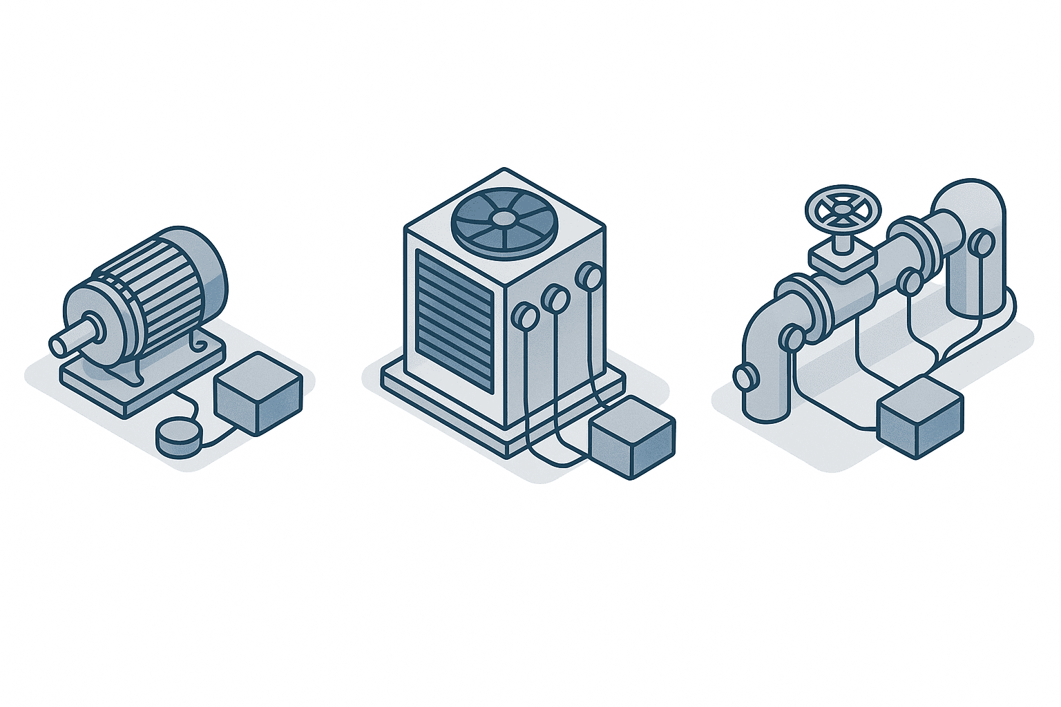
There is exactly one condition under which predictive maintenance is possible. Some measurable physical quantity has to change before the failure occurs. Attach anything you like to equipment where that condition does not hold and you will not predict anything. And which physical quantity changes, how far in advance it changes, and how clearly it changes are all fundamentally determined by the equipment type. That is where the three patterns come from.
| Aspect | Pattern A | Pattern B | Pattern C |
|---|---|---|---|
| Target equipment | Rotating equipment, meaning motors, pumps and conveyors | Refrigeration equipment, meaning chillers and refrigeration units | Continuous process equipment, meaning a concentration and sterilisation line |
| Physical quantity measured | Vibration, in acceleration and velocity | A combination of temperature, pressure and current | Multi-point temperature, pressure and flow data |
| Analysis method | Frequency analysis using FFT and envelope analysis | Machine learning anomaly detection | Causal analysis AI across multiple variables |
| How the abnormality appears | Clearly, in a single physical quantity | In a combination of several values | As a breakdown in the relationships between variables |
| Maturity of the technology | Well established | Practical and in use | Requires specialist involvement |
| Where the difficulty sits | Mounting position and threshold setting | Handling seasonal ambient temperature swing | Defining what normal actually is |
Why Pattern A has the most case studies behind it
Failures in rotating equipment, meaning bearing wear, shaft misalignment and imbalance, show up in vibration with unusual honesty, and vibration is a single physical quantity. On top of that, once you know the rotational speed you can map frequency components to specific components of the machine on theoretical grounds. That is what makes thresholds possible and what allows the type of failure to be inferred, not just its presence. The reason the world’s published predictive maintenance case studies skew so heavily towards rotating equipment is this physical straightforwardness, not the idea that rotating equipment is the most important thing in a plant.
There is, however, a clear boundary between the failures vibration can see and the failures it cannot. That boundary sits outside the scope of this article, so please refer to the breakdown in our article on equipment diagnosis with vibration sensors. It becomes necessary once you have decided on Pattern A and are working out which failure modes you are actually targeting.
Pattern B gets harder because Thailand has seasons
Degradation in a chiller or a refrigeration unit does not appear in a single physical quantity. Refrigerant leakage, condenser fouling and falling compressor efficiency all appear as a combination of several values, namely current consumption creeping up, the pressure differential widening, and the unit taking longer to reach its setpoint. That is why the method used here is machine learning anomaly detection, meaning you train a model on data from normal operation and detect departures from it.
This is where a difficulty specific to Pattern B appears. A chiller’s current consumption depends heavily on ambient temperature. In an environment like Thailand, where conditions differ substantially between the dry season and the rainy season, the observation that current has risen tells you nothing on its own about whether the cause is degradation or the weather. The training data therefore has to span the seasons, and the effort of building the model is greater than in Pattern A. That effort shows up as the third cost layer in the investment breakdown below.
Pattern C starts by defining what normal actually means
Abnormalities in continuous process equipment such as a concentration line or a sterilisation line appear neither as vibration nor as a single temperature or pressure reading. What appears is something like the temperature rising while the concentration fails to rise as expected, or the flow rate staying constant while pressure loss increases. In other words, a breakdown in the relationships between variables. Detecting that requires sensors at many points and an analysis capable of capturing the causal structure among them.
What makes this pattern awkward is that the normal state itself changes with product grade and batch conditions. Put anomaly detection on equipment whose normal state has never been defined and you get a pile of false alarms, after which the floor learns to ignore the alarms entirely. The reason Pattern C’s investment includes a line item for specialist tuning is that this definition work has to be done by someone.
Sorting your own equipment against three criteria
Before you read another case study, rank your own equipment against the three criteria below. Once that sorting is done, which case studies apply to you is decided automatically.
| Criterion | What to check on the floor | How it drives pattern selection |
|---|---|---|
| Frequency | How many unplanned stoppages does this equipment class have per year | Low frequency stretches the payback period |
| Loss per event | When it stops once, how much is lost including scrap, repair and overtime | Multiplied by frequency, this sets the order of attack |
| Detectability | Can you explain which physical quantity changes before the failure, and how | Sensors on equipment you cannot explain will not detect anything |
Skipping the third criterion and pressing on is the most common failure of all. Decide your starting equipment from frequency and loss alone and the high-value equipment rises to the top of the list. But there is no guarantee that failures in that equipment appear in any measurable physical quantity. What that mix-up actually costs is shown in money in the mismatch calculation later in this article.
Pattern A, Vibration Monitoring for Rotating Equipment, an Established Method and What It Costs
The configuration here places vibration sensors on all 90 pieces of rotating equipment in the model factory and uses frequency analysis to catch the precursors of bearing degradation and misalignment. It is the most technically established of the three patterns, and because the unit count is high, unit prices have a large effect on the total.
The investment, layer by layer
| Layer | Content | Amount (THB) | Basis |
|---|---|---|---|
| Layer 1 | Vibration sensors | 1,080,000 | 90 units x 12,000 THB |
| Layer 2 | Installation work | 270,000 | 90 units x 3,000 THB |
| Layer 3 | Initial licence for the frequency analysis software and threshold setting | 180,000 | Lump sum |
| Layer 4 | Gateways and communications equipment | 150,000 | Lump sum |
| Layer 5 | Training and operating documentation | 120,000 | Lump sum |
Total investment is 1,800,000 THB. Because the unit count is high, layers 1 and 2, meaning the costs that scale with physical volume, make up most of the total. Put the other way round, narrow the scope and the investment falls in direct proportion. You do not have to instrument all 90 units at once, and the ability to expand in stages, starting from the equipment with the largest product of frequency and loss per event, is Pattern A’s main practical advantage.
Annual operating cost consists of sensor maintenance at 90 units x 1,500 THB per year, giving 135,000 THB, plus the analysis software licence at 120,000 THB, for a total of 255,000 THB.
Benefit and payback
Assume that catching vibration precursors converts 6 of the 8 annual unplanned failures into planned stoppages. Two unplanned failures remain, so the residual loss is 2 events x 145,000 THB, which is 290,000 THB. The annual reduction is 1,160,000 THB minus 290,000 THB, giving 870,000 THB.
Net benefit is the 870,000 THB reduction minus the 255,000 THB of annual operating cost, giving 615,000 THB. Payback is the 1,800,000 THB investment divided by that net benefit of 615,000 THB, which is 2.93 years.
The phrase about converting failures into planned stoppages is doing real work in that paragraph. Predictive maintenance is not a technology that makes failures disappear. It is a technology that moves the timing of a failure to a moment that suits you. The same bearing replacement costs a different amount depending on whether it happens as an emergency call-out at two in the morning or as a scheduled swap during a planned shutdown, in overtime and in the premium paid to source a part in a hurry. That is precisely why the 145,000 THB avoided is made up of production stoppage, emergency repair and overtime.
If your plant has a lot of older equipment and there is no prepared mounting face or cable route for a sensor, additional installation cost appears. The cost structure of retrofitting sensors onto existing equipment is broken into five layers in our article on IoT retrofit for legacy equipment, so if your equipment is old, take those figures and add them on top of layer 2 here.
Pattern B, Composite Monitoring Plus AI Anomaly Detection for Chillers, and How to Handle Seasonal Swing
This configuration places composite temperature, pressure and current sensor kits on the 8 pieces of refrigeration equipment and runs machine learning anomaly detection on top of them. Although there are only 8 units, both the sensor kit and the installation work per unit sit a clear step above Pattern A’s unit prices of 12,000 THB for the sensor and 3,000 THB for installation.
The investment, layer by layer
| Layer | Content | Amount (THB) | Basis |
|---|---|---|---|
| Layer 1 | Composite temperature, pressure and current sensor kits | 680,000 | 8 units x 85,000 THB |
| Layer 2 | Installation work | 200,000 | 8 units x 25,000 THB |
| Layer 3 | Initial machine learning model build and preparation of training data spanning the seasons | 450,000 | Lump sum |
| Layer 4 | Gateways and communications equipment | 80,000 | Lump sum |
| Layer 5 | Training and operating documentation | 60,000 | Lump sum |
Total investment is 1,470,000 THB. The structural difference from Pattern A shows up most clearly in layer 3, which swells from 180,000 THB in Pattern A to 450,000 THB here. As described in the previous section, unless variation caused by ambient temperature is learned as normal variation, the alarms will start firing continuously the moment the dry season arrives.
Annual operating cost consists of sensor maintenance at 8 units x 8,000 THB per year, giving 64,000 THB, plus annual model retraining and maintenance at 140,000 THB, for a total of 204,000 THB. There is another difference from Pattern A here. Pattern A’s operating cost is mostly a software licence, whereas Pattern B carries a budget line that assumes the model is rebuilt every year. Any configuration that uses machine learning is not a fit-and-forget installation. It requires an ongoing operation that keeps updating the model as the equipment ages and as operating conditions change.
Benefit and payback
Assume the 3 unplanned failures a year fall to 1. The residual loss is 1 event x 380,000 THB, which is 380,000 THB, and the annual reduction is 1,140,000 THB minus 380,000 THB, giving 760,000 THB.
Net benefit is 760,000 THB minus 204,000 THB, giving 556,000 THB, and payback is 1,470,000 THB divided by 556,000 THB, which is 2.64 years. That is faster than Pattern A’s 2.93 years.
Only 8 units are covered and only 2 failures a year are eliminated, yet payback is faster than Pattern A across 90 units. The reason is the 380,000 THB loss per event doing the work. A refrigeration failure costs more in scrapped product than in repairs. Inventory that has been through a temperature excursion does not come back once the equipment is fixed. Return on investment is decided by the weight of a single event, not by the number of units, and that is the character of Pattern B.
Pattern C, Causal Analysis AI for Continuous Process Equipment, Hard to Detect but Expensive per Event
This configuration adds 20 temperature, pressure and flow measurement points to the single concentration and sterilisation line and uses causal analysis AI to catch precursors in the correlations among multiple variables. Only one line is covered, yet the investment is the largest of the three patterns.
The investment, layer by layer
| Layer | Content | Amount (THB) | Basis |
|---|---|---|---|
| Layer 1 | Additional temperature, pressure and flow sensors | 900,000 | 20 points x 45,000 THB |
| Layer 2 | Wiring and installation work | 380,000 | Lump sum |
| Layer 3 | Initial causal analysis AI licence and model build | 1,250,000 | Lump sum |
| Layer 4 | Data platform build and specialist tuning | 420,000 | Lump sum |
| Layer 5 | Training and building the operating organisation | 210,000 | Lump sum |
Total investment is 3,160,000 THB. This is the only one of the three patterns where the analysis side costs more than the sensors themselves. Layer 3 at 1,250,000 THB plus layer 4 at 420,000 THB gives an analysis-related total that exceeds the 900,000 THB of layer 1 sensors.
That structure becomes an argument every time the estimate goes into a cost-reduction round. Sensors and installation leave something physical behind and are accepted readily, while model building and tuning leave nothing visible and are therefore the first items on the chopping block. But cut layers 3 and 4 out of Pattern C and what remains is a set of sensors that detect nothing. Abnormalities in continuous process equipment appear as a breakdown in the relationships between variables, so collecting data is not the same thing as detecting anything. If something has to be cut, narrowing the target process and reducing the number of measurement points is the structurally healthier option.
Annual operating cost consists of sensor maintenance at 20 points x 3,000 THB per year, giving 60,000 THB, plus the continuing AI licence at 320,000 THB, for a total of 380,000 THB.
Benefit and payback
Assume the 2 unplanned stoppages a year fall to 0.5, meaning roughly one every two years. The residual loss is 0.5 events x 920,000 THB, which is 460,000 THB, and the annual reduction is 1,840,000 THB minus 460,000 THB, giving 1,380,000 THB.
Net benefit is 1,380,000 THB minus 380,000 THB, giving 1,000,000 THB, and payback is 3,160,000 THB divided by 1,000,000 THB, which is 3.16 years.
Putting the three patterns in one frame

Here are the three patterns compared on identical terms. Every figure is a model factory estimate.
| Item | Pattern A, rotating equipment and vibration | Pattern B, chillers with composite sensing and AI | Pattern C, process equipment and causal analysis AI |
|---|---|---|---|
| Target | 90 units of rotating equipment | 8 units of refrigeration equipment | 1 continuous process line |
| Investment (THB) | 1,800,000 | 1,470,000 | 3,160,000 |
| Annual operating cost (THB) | 255,000 | 204,000 | 380,000 |
| Change in unplanned failures | 8 to 2 per year | 3 to 1 per year | 2 to 0.5 per year |
| Residual loss (THB) | 290,000 | 380,000 | 460,000 |
| Annual reduction (THB) | 870,000 | 760,000 | 1,380,000 |
| Net benefit (THB) | 615,000 | 556,000 | 1,000,000 |
| Payback | 2.93 years | 2.64 years | 3.16 years |
There are three things to read out of that table.
First, all three patterns land inside a payback range of 2.64 to 3.16 years, and none of them is decisively superior. As long as the pattern is matched to the equipment type, all three stand up as investments. Neither the claim that predictive maintenance only works on rotating equipment nor the claim that AI-based configurations produce bigger benefits survives contact with this table.
Second, the largest net benefit in absolute terms belongs to Pattern C at 1,000,000 THB. But its investment is also the largest at 3,160,000 THB, and its payback is the slowest. Decide your order of attack by looking only at annual savings and you will begin with the pattern that costs the most and demands the most specialist involvement.
Third, the fastest payback belongs to Pattern B, which covers 8 units against Pattern A’s 90. Spending 1,470,000 THB on 8 chillers looks expensive next to 1,800,000 THB on 90 pieces of rotating equipment, yet it pays back in 2.64 years against 2.93. Investment efficiency is not decided by how many units are in scope.
One boundary is worth stating. Where the data detected by these three patterns gets consolidated, and how it connects to maintenance work orders and spare parts inventory, is outside the scope of this article. Deploy anomaly detection while work management stays on paper and you end up in a state where alarms fire but nobody can trace who responded and when. We cover that in our article on choosing an equipment maintenance management system. Separately, the implementation sequence and detailed costing for what to do after you have chosen a single pattern is set out in our guide to deploying a predictive maintenance system, so once this article has helped you settle on a pattern, read that one next.
Predictive Maintenance at Real Companies, an Automotive Stamping Plant, Unilever, JFE Chemical and Nippon Steel
Everything up to this point has been a model factory estimate. From here we look at published cases from real companies. The currencies, the scale and the underlying assumptions are all different, so read this section separately from the Thai baht estimates above. The useful way to read them is to ask which of the three patterns each case most closely resembles, because that is what makes them transferable to your own plant.
An automotive stamping plant, catching hydraulic component degradation early
An automotive stamping plant with 200 employees instrumented 12 hydraulic presses with sensors. In this plant’s case, the investment was $145,000. Within 8 months of go-live it detected hydraulic seal degradation in advance on 3 of the presses and avoided emergency stoppage and repair costs of roughly $180,000 per event. First-year ROI was reported at 3.7 times.
What this case demonstrates is that a scope as small as 12 machines still works, provided the avoided cost of a single event exceeds the investment. It has the same character as the structure described under Pattern B, where the weight of one event decides the outcome rather than the number of units.
Unilever’s Indaiatuba plant in Brazil, what large-scale deployment looks like at the far end
Unilever’s plant in Indaiatuba, Brazil, deployed more than 50,000 IoT sensors. In Unilever’s case, this achieved annual savings of $2.3 million, including a 45% reduction in maintenance costs, and the $1.2 million investment was reported as recovered in under 7 months.
A scale of 50,000 sensors is not the level most Japanese-owned factories should be aiming for on day one. The important thing when reading this case is not the savings figure but how many stages it took to reach that scale. Handling data from 50,000 sensors requires the collection platform, the model operations organisation and the floor-level response process for alarms to have grown up together. The practical way to treat this case is as a destination to reference, not as an architecture to target from the start.
JFE Chemical, converting reboiler fouling into a planned shutdown
JFE Chemical had previously dealt with fouling in a distillation column reboiler only after the fact. By deploying Brains Technology’s anomaly detection solution Impulse, the company was able to identify the timing for cleaning and shutdown in advance and convert the event into a planned stoppage.
This is the case that most closely resembles Pattern C in this article. Fouling in a distillation column does not appear in vibration. There is no route to it other than reading the trend in process state variables, and even when you can detect that fouling is progressing, whether that means the unit has to be stopped immediately is a separate judgement. The value created in this case did not come from preventing a failure. It came from being able to pull the timing of a shutdown into the company’s own plan.
Nippon Steel, validating detectability on equipment that used to take 10 days to diagnose
Nippon Steel had previously needed 10 days to determine the root cause of complex equipment troubles. After deploying NEC’s Invariant Analysis, the company confirmed that for past troubles, early detection would have been possible using offline data.
The point worth noticing in this case is the sequence. The company did not put the system straight into live operation. It validated detectability against historical data first. In a configuration like Pattern C, where the investment is large and the work begins with defining the normal state, skipping that validation step is how the money gets spent on nothing. If you still hold historical records, confirming whether precursors are visible in that history is a far safer path than adding sensors first.
The benefit levels reported in general surveys
Alongside individual cases, the benefit levels reported across multiple surveys are also worth having in view. Several deployments of AI-driven predictive maintenance report ROI of 300% to 500% and payback within 6 to 18 months (Tech-Stack, 2025). Plants making full use of AI-driven predictive maintenance are reported to have cut unplanned downtime by 30% to 50% and extended equipment service life by 20% to 40% (McKinsey, 2025).
Set those numbers against the model factory’s estimates, which pay back in 2.64 to 3.16 years, and the model factory is clearly the more conservative of the two. Two reasons are plausible. One is that the model factory assumes residual failures after deployment of 2, 1 and 0.5 events a year rather than zero, and derives payback from a net benefit that already has operating cost deducted. The other is that figures from plants which have reached full utilisation of the technology cannot be compared like for like with figures for a plant that is about to begin. Read the numbers in published case studies as the ceiling in a case that went well, and build your own estimate up from your own failure history.
What Happens When Equipment Type and Pattern Are Mismatched, a Costed Example

We have repeated throughout this article that the pattern has to be matched to the equipment type. So what happens when it is not. Here it is in money.
The case we model is Pattern A, meaning vibration sensors, transplanted directly onto continuous process equipment. This is not a hypothetical. It is a genuinely likely choice. Vibration sensors have the most case studies behind them and are the easiest configuration to explain internally. After rotating equipment produces results, the natural next move is to say that the same approach should be extended to the rest of the plant.
The problem is that abnormalities in continuous process equipment do not appear as vibration. Temperature drift, changes in concentration, a shift in how far a reaction has progressed. None of that reaches an accelerometer bolted to the outside of a pipe. What you get is a state in which the sensors work correctly, the data is being collected, and the precursors of the abnormality sit entirely outside the detection envelope.
| Item | Pattern C, matched to the equipment | Mismatch, vibration sensors transplanted |
|---|---|---|
| Investment (THB) | 3,160,000 | 650,000 |
| What the investment buys | 20 sensor points, causal analysis AI, and platform build | 20 points x 30,000 THB for vibration sensors plus 50,000 THB installation |
| Annual operating cost (THB) | 380,000 | 30,000 |
| Change in unplanned stoppages | 2 to 0.5 per year | 2 to 1.9 per year |
| Residual loss (THB) | 460,000 | 1,748,000 |
| Annual reduction (THB) | 1,380,000 | 92,000 |
| Net benefit (THB) | 1,000,000 | 62,000 |
| Payback | 3.16 years | 10.48 years |
The mismatched option costs 650,000 THB, far less than Pattern C’s 3,160,000 THB. Its annual operating cost is light too, at 30,000 THB. It is an easy proposal to get approved. But its annual reduction is only 92,000 THB, because 2 unplanned stoppages a year become 1.9, which in practical terms is no reduction at all. Net benefit stops at 62,000 THB and payback comes out at 10.48 years.
On the same equipment, the right pattern pays back in 3.16 years and the wrong one in 10.48. Even though the investment has been cut dramatically, the payback period deteriorates by more than a factor of three. What this contrast shows is that the cheaper option is not automatically the more efficient one.
What makes this failure mode awkward is how late it surfaces. The sensors are running, data is accumulating, and waveforms are showing on the dashboard. Because nothing is visibly broken, nobody registers it as a problem. By the time somebody notices, one or two years later, that stoppages on this equipment never actually went down, the money has been spent and the operating routine has settled around it.
There is exactly one way to avoid this. Before you choose a sensor, take several failures that genuinely happened in the past and check whether you can explain what changed first on each occasion. If you can explain it, choose a sensor that measures that quantity. If you cannot, that equipment is not yet a candidate for predictive maintenance, and the right stage for it is collecting data to establish what its normal state looks like. Validating against historical data first, as Nippon Steel did, is exactly this piece of work.
Sensitivity Analysis, How Payback Moves When the Assumptions Break
Every payback figure above rests on assumptions. Here we check, pattern by pattern, whether the conclusion changes when those assumptions break. One important note first. Each of the three cases below applies to one pattern only and has no effect on the others. Apply a single coefficient uniformly across all three patterns and the conclusion will swing much further than reality warrants.
| Case | Assumption that breaks | Applies to | Net benefit (THB) | Payback |
|---|---|---|---|---|
| Base | Assumptions hold | Pattern A | 615,000 | 2.93 years |
| Case 1 | Detection accuracy is lower, so failures fall only from 8 to 4 per year | Pattern A | 325,000 | 5.54 years |
| Base | Assumptions hold | Pattern B | 556,000 | 2.64 years |
| Case 2 | Loss per event is actually half, at 190,000 THB | Pattern B | 176,000 | 8.35 years |
| Base | Assumptions hold | Pattern C | 1,000,000 | 3.16 years |
| Case 3 | The plant only has 1 unplanned stoppage a year to begin with | Pattern C | 80,000 | 39.5 years |
Case 1, detection accuracy is lower than assumed, applying to Pattern A
This is the case where vibration monitoring detects less than expected and the 8 unplanned failures a year fall only to 4 rather than 2. Residual loss is 4 events x 145,000 THB, which is 580,000 THB, and the annual reduction is 1,160,000 THB minus 580,000 THB, giving 580,000 THB. Net benefit is 580,000 THB minus the 255,000 THB of operating cost, giving 325,000 THB, and payback is 1,800,000 THB divided by 325,000 THB, which is 5.54 years. That is 89% longer than the base case of 2.93 years.
Payback nearly doubles, but the investment does not stop being viable. Pattern A rests on well-established technology, and there is room to improve accuracy after the fact by revisiting mounting positions and thresholds. The sensible way to take 5.54 years is that, depending on your internal hurdle rate, it lands on the borderline.
Case 2, the loss estimate was too high, applying to Pattern B
This is the case where the 380,000 THB estimate for a single refrigeration failure was overstated and the real figure is half of it, 190,000 THB. The current annual loss becomes 3 events x 190,000 THB, which is 570,000 THB, the residual loss after deployment becomes 1 event x 190,000 THB, which is 190,000 THB, and the reduction becomes 380,000 THB. Net benefit is 380,000 THB minus the 204,000 THB of operating cost, giving 176,000 THB, and payback is 1,470,000 THB divided by 176,000 THB, which is 8.35 years. That is a severe deterioration from the base case of 2.64 years.
The reason Pattern B had the fastest payback in the base case was that the 380,000 THB loss per event was doing the work. Turned around, that means Pattern B’s payback depends heavily on the accuracy of that one estimate. Getting it closer to reality requires knowing the actual value of the product you have scrapped. In a plant with no record of the value of inventory discarded after past temperature excursions, that number becomes a guess, and the uncertainty in the payback period stays there unresolved. The first number a plant considering Pattern B should check is not a sensor specification, it is the history of what has been scrapped.
Case 3, a plant where failures are rare to begin with, applying to Pattern C
This is the case where the continuous process line suffers 1 unplanned stoppage a year rather than 2. Here the baseline loss itself changes. The current annual loss becomes 1 event x 920,000 THB, which is 920,000 THB, the residual loss after deployment becomes 0.5 events x 920,000 THB, which is 460,000 THB, and the reduction is 460,000 THB. Net benefit is 460,000 THB minus the 380,000 THB of operating cost, giving 80,000 THB, and payback is 3,160,000 THB divided by 80,000 THB, which is 39.5 years.
At 39.5 years there is no investment case at all. A plant in this position should not start with Pattern C. Because continuous process equipment carries a large loss per event, it feels like the obvious first priority. But the only failures you can remove are the ones actually happening, and removing 0.5 events a year from equipment that was only stopping once a year will never repay 3,160,000 THB.
Decide the order of attack from measured frequency multiplied by loss
What the three cases have in common is that the order of attack must not be decided by a felt sense of how important each piece of equipment is. Pattern C looks attractive because its loss per event is large, yet in a plant with low failure frequency its payback collapses. Pattern A, conversely, stands up despite a small loss per event, because a frequency of 8 events a year carries it.
So there are only two inputs that decide the order of attack. The count of unplanned stoppages by equipment class over the past several years, and the real cost of a single event including scrap, repair, overtime and emergency substitution. Rank by the product of those two, then work down the list checking detectability. Follow that order and you can reach a decision simply by substituting your own values into the tables in this article.
What to Know Before Evaluating Predictive Maintenance in a Thai Factory
If you are evaluating predictive maintenance for a Japanese-owned plant in Thailand, several assumptions carried over from Japanese case studies will not hold. This is not about the technology. It is about operating conditions and the state of the equipment.
Equipment age and what it takes to mount a sensor
It is common in Japanese-owned plants in Thailand to find equipment relocated from the parent plant in Japan still in active service. Relocated equipment often has drawings that were never updated, or a modification history that never made it to the local site. When the time comes to fit a vibration sensor, problems surface at the installation stage, such as there being no usable mounting face at all, or no spare space in the control panel for an addition.
That cost is included in layer 2 of the investment breakdowns above, but the model factory assumes standard conditions. In plants with older equipment, that layer can exceed the assumption. Where the additions land and how large they get is covered in our article on IoT retrofit for legacy equipment, so check it against the condition of your own equipment before you start.
Ambient conditions and seasonal variation
As noted under Pattern B, current consumption in chillers and refrigeration units depends on ambient temperature. Under Thai climate conditions, the annual range of ambient temperature affects the training data, so the estimate of how long model building takes differs from Japanese case studies. A model trained only on dry season data behaves differently once the rainy season starts. If you choose Pattern B, build the time it takes for the model to stabilise into the plan.
Whether your maintenance records still exist
Every estimate in this article starts from two numbers, namely the count of past unplanned stoppages and the loss per event. In a plant where neither has been recorded, the estimate cannot be made at all. What we see most often in practice is a plant that has kept its repair records but never linked them to downtime duration or to the value of what was scrapped. In that situation, structuring the maintenance records first is a better investment than starting predictive maintenance, because once the records are structured, which equipment class to start with becomes visible on its own. How to manage maintenance records is covered in our article on choosing an equipment maintenance management system.
Who will run it locally
Predictive maintenance does not end at go-live. Pattern A needs thresholds revisited, Pattern B needs annual model retraining, and Pattern C needs continuing tuning. That is exactly why the model factory carries annual operating costs of 255,000 THB for Pattern A, 204,000 THB for Pattern B and 380,000 THB for Pattern C. Unless you decide up front whether the local maintenance team runs this, whether the Japanese head office monitors it remotely, or whether it goes to an external provider, you end up with alarms that nobody looks at. In fact, we suspect that the figures quoted at the top of this article, 65% planning against 32% executing, are less a statement about technology than a statement about this question of ownership going unanswered.
Summary, Start by Sorting Your Own Equipment Into Patterns
Here is the conclusion. Predictive maintenance is not a technology you decide on by asking whether to adopt it. What decides the return is whether, class by class, you have confirmed which physical quantity carries the precursor of failure and then matched a detection pattern to it.
In the model factory’s estimates, Pattern A, vibration monitoring across 90 pieces of rotating equipment, costs 1,800,000 THB and pays back in 2.93 years. Pattern B, composite monitoring with AI anomaly detection on 8 refrigeration units, costs 1,470,000 THB and pays back in 2.64 years. Pattern C, causal analysis AI on one continuous process line, costs 3,160,000 THB and pays back in 3.16 years. As long as the pattern matches the equipment, all three stand up as investments.
The mismatched case, transplanting vibration sensors onto continuous process equipment, holds the investment down to 650,000 THB, yet the annual reduction stops at 92,000 THB and payback deteriorates to 10.48 years. Cheap is not the same as efficient.
The sensitivity analysis then showed that a plant with only 1 unplanned stoppage a year that starts with Pattern C is looking at a payback of 39.5 years. Equipment with a large loss per event feels like the obvious priority, but the only failures you can remove are the ones that are actually happening.
With that established, there are three numbers we would ask you to measure before you begin. The first is the annual count of unplanned stoppages by equipment class. The second is the real cost of a single event, including scrap, repair, overtime and emergency substitution. The third is whether you can explain what changed first in your past failures. The third is the one most often skipped and the one that costs the most. Once you have all three, you can decide which pattern to apply to which equipment simply by substituting your own values into the tables in this article.
Talking It Through While You Are Still Evaluating
Which of the three patterns your equipment falls into, and whether it is a candidate for predictive maintenance at all, cannot be settled from specifications alone. It takes a session looking at your past failure records together and working out what changed first on each occasion. TOMAS TECH supports production management and OT/IoT deployment for Japanese-owned factories in Thailand, and it is fine to talk to us even if you are not yet sure which pattern fits your equipment. It is entirely acceptable to come to us only wanting to see what the tables in this article look like with your own failure history in them. Please get in touch here whenever it suits you.
Frequently Asked Questions
What patterns do predictive maintenance case studies fall into
Broadly three. The first fits vibration sensors to rotating equipment, meaning motors, pumps and conveyors, and uses frequency analysis to catch bearing degradation and misalignment. It has the most case studies behind it and the technology is well established. The second fits composite temperature, pressure and current sensors to chillers and refrigeration units and uses machine learning to detect departures from the normal state. The third adds sensors at many points on continuous process equipment and uses causal analysis AI to catch breakdowns in the relationships between variables. When you read a case study, check which equipment class the company applied which pattern to. A case study that does not tell you cannot be used to reason about your own plant.
What equipment suits predictive maintenance and what equipment does not
It suits equipment where a measurable physical quantity changes before the failure occurs, and where the product of stoppage frequency and loss per event is large. It does not suit equipment where you cannot explain what changes before a failure, or equipment that barely suffers unplanned stoppages in the first place. In the model factory’s sensitivity analysis, a plant whose continuous process equipment stops only once a year would face a payback of 39.5 years if it started with Pattern C. Equipment with a large loss per event looks like the top priority, but predictive maintenance can only reduce failures that are actually occurring, and it cannot get ahead of failures that are not happening. Decide the order of attack from measured frequency and loss.
What is the difference between predictive maintenance and condition-based early detection
In practice the two terms are used almost interchangeably. Both refer to a maintenance approach that monitors equipment condition continuously, catches the signs of an abnormality and acts before the failure. If you want to separate them, early detection puts its weight on detecting the sign of an abnormality, while predictive maintenance sometimes carries the further implication of forecasting when the failure will occur and building that into a plan. That distinction shifts with context, though, so rather than arguing about terminology it is more useful in practice to check what a given method measures and what it detects. The distinction that actually matters for an investment decision is the one against run-to-failure, meaning fixing it after it breaks, and time-based maintenance, meaning replacing on a fixed interval.
How much does deploying predictive maintenance cost
It changes by an order of magnitude depending on the pattern. In the model factory’s estimates, Pattern A across 90 pieces of rotating equipment came to 1,800,000 THB, made up of 1,080,000 THB for sensors, 270,000 THB for installation, 180,000 THB for analysis software, 150,000 THB for gateways and 120,000 THB for training. Pattern B across 8 refrigeration units came to 1,470,000 THB, and Pattern C on one continuous process line came to 3,160,000 THB. Annual operating costs are 255,000 THB, 204,000 THB and 380,000 THB respectively. Pattern A scales with unit count, so narrowing the scope brings the figure down proportionally, whereas Pattern C is dominated by analysis-side cost and narrowing the scope will not move it much. The cost breakdown and the deployment sequence are set out in our guide to deploying a predictive maintenance system.
Can predictive maintenance be deployed on old existing equipment
Age on its own is not an obstacle. Vibration, temperature and pressure can be measured regardless of the year the machine was built. What does become an issue is the mounting conditions, meaning whether a mounting face can be secured for the sensor, whether the control panel has room for an addition, and how the cable route will be run. In Japanese-owned plants in Thailand it is common to find equipment relocated from the parent plant still in service, sometimes with no drawings or modification history held locally. In that situation, layer 2 of the estimates in this article, meaning installation work, can exceed the assumption. The cost structure of retrofitting sensors onto ageing equipment is set out in our article on IoT retrofit for legacy equipment, so please check it before you start.
References
- Predictive maintenance case studies and reported ROI levels using AI, covering the automotive stamping plant, Unilever’s Indaiatuba plant, and survey figures from Tech-Stack, McKinsey and MaintainX, IIoT World, confirmed as of August 2026
- Global predictive maintenance market size and the manufacturing share of that market, Coherent Market Insights, confirmed as of August 2026
- Predictive maintenance deployments at JFE Chemical and Nippon Steel, in Japanese, IT trend manufacturing DX, confirmed as of August 2026