



In factories that have been live on an MRP system for six months to a year, we hear almost exactly the same sentence: “nobody believes the calculation results.” Order proposals are printed every day, yet the buyer recalculates them in their own Excel file, production control phones the shop floor to confirm stock, and in the end the parts get arranged by the same human intuition that ran the plant before go-live. The implementation project was signed off as a success, and yet only the results have disappeared.
At this point the suspicion usually falls on the software: “the calculation engine does not fit our production model,” or “we picked the wrong product.” When you take the operation apart, however, the cause is almost never there. MRP is a simple subtraction machine that takes three master data sets as its input, and what stops is not the calculation but the freshness of the master data on the input side. What is more, those three go stale at three different speeds. And a plant in Thailand carries a fourth master that the head office in Japan never assumed.
This article breaks down the structure of an MRP that does not run, using figures grounded in the reality of Japanese-affiliated manufacturers with plants in Thailand. In particular, it walks through the intermediate arithmetic behind two points: how an item-level BOM accuracy of 98%, a number that does not look bad at all, turns into 49% at the product level, and the double counting of inventory reduction that appears in almost every capital request.
What an MRP system actually calculates: the input is only three master data sets
MRP, or Material Requirements Planning, has a grand-sounding name but does something extremely simple.
From the gross requirement of “what is needed, how many, and when,” it subtracts “what we hold right now” and “what is already on order and due to arrive,” and then orders the shortfall at a timing that still makes the date. That is all. Written as a formula: net requirement = gross requirement – on-hand stock – scheduled receipts + allocated quantity.
The catch is that every input to that subtraction comes from master data. Specifically, from the following three.
| Input master | What MRP uses from it | What happens when it drifts |
|---|---|---|
| On-hand stock | Actual quantity per item, allocated quantity, scheduled receipts | The subtrahend is wrong. You order what you already have, and fail to order what you do not have |
| Bill of materials (BOM) | Component parts and quantity per unit of product | The multiplier is wrong. Missed orders and dead stock appear at the same time |
| Lead time and order lot | Procurement lead time, minimum order quantity, order multiples | Order timing and order quantity are wrong. Parts arrive too late, or in a quantity you will never consume |
When MRP explodes the gross requirement, it multiplies the production plan by the BOM. Get the multiplication wrong and the required quantity is off across the board. Stock is then subtracted from that, so a wrong stock figure produces a wrong order quantity. Finally the order date is back-calculated with the lead time, so a stale lead time produces a wrong date. In other words, the correctness of MRP output is the product of the correctness of three master data sets. If any one of them collapses, the output is unusable no matter how refined the other two are.
Once that is clear, one common misconception disappears: the idea that “installing an MRP system reduces inventory.” MRP has no function that reduces inventory. What it has is a function that calculates requirements and makes shortages and excesses visible. Inventory falls only when that calculation has become trustworthy enough for the plant to thin out the insurance policy it calls safety stock. If the master data stays stale, MRP becomes a machine that mass-produces untrustworthy results every day, and the shop floor builds up manual insurance stock to cancel them out. That is the route by which some factories end up with more inventory after go-live, not less.
Typical patterns in which a production management system fails to deliver what was expected are organised in why production management system implementations fail. For MRP specifically, the centre of gravity of failure sits clearly on the master data side.
The real reason an MRP system does not run: all three masters age at different speeds
An implementation project brings all three master data sets into a “correct state” on the same day. The BOM is reviewed item by item, a physical count aligns stock, and suppliers are asked to confirm their latest lead times. On cut-over day, the three masters really are correct.
The problem starts the next day. The three begin to age at separate speeds, and the gap between those speeds is exactly what hides the decay.
At one Japanese-affiliated component maker in Thailand, referred to below as our model factory, the drift of the three masters was measured one year after go-live. The result is as follows.
| Master | Actual changes per year | Not reflected in the system | Drift rate |
|---|---|---|---|
| Bill of materials (BOM) | 210 design changes | 42 | 20.0% |
| Inventory | Count of 620 items | 74 items with discrepancies | 11.9% |
| Lead time and order lot | 96 supplier changes | 75 | 78.1% |
The arithmetic is 42 / 210 = 20.0%, 74 / 620 = 11.9%, and 75 / 96 = 78.1%.
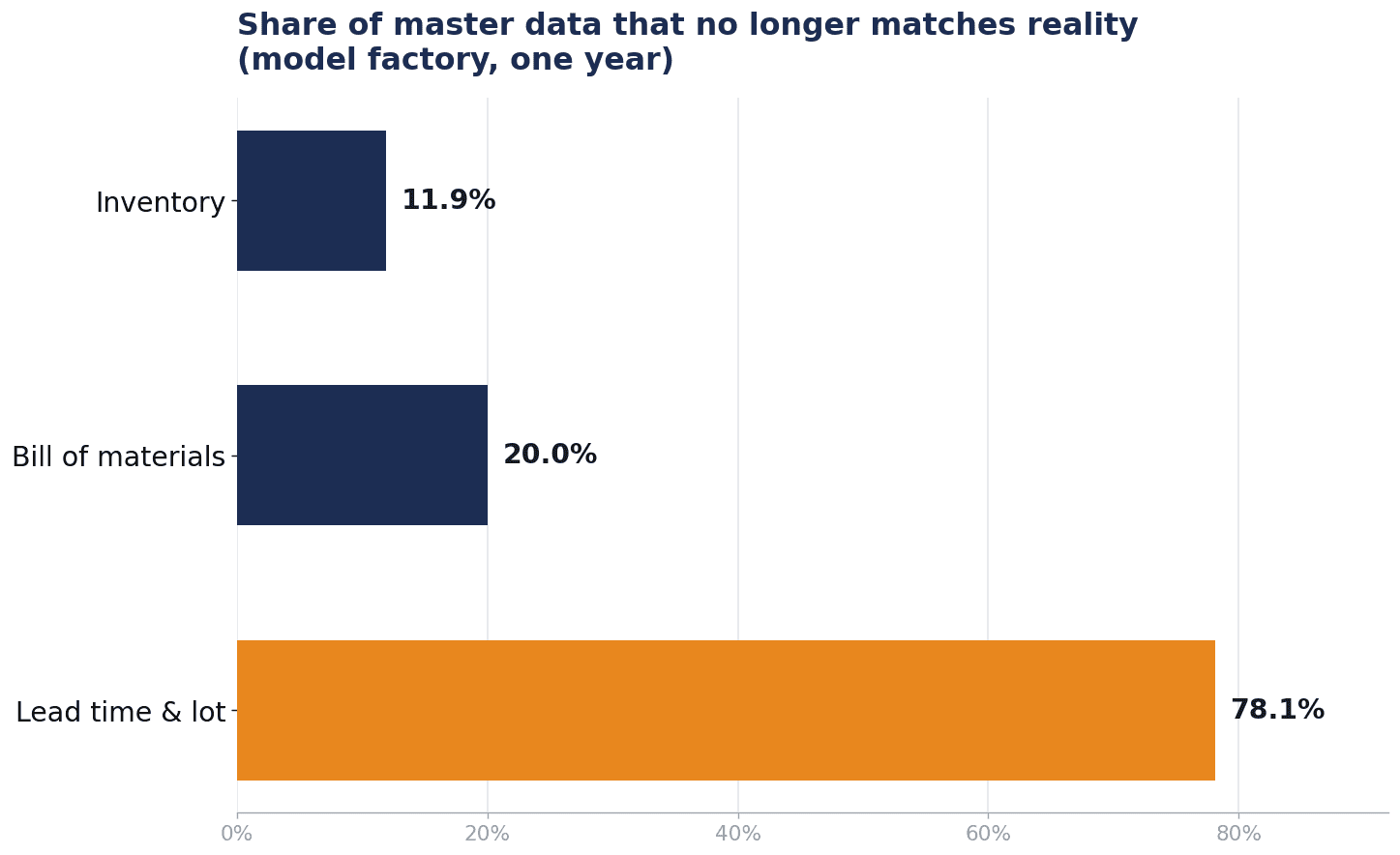
The stalest master is lead time and order lot, the one nobody has been made responsible for updating
Show this table to plant managers and most of them react first to the 20.0% on the BOM. The genuinely dangerous number, however, is the 78.1%. Let us take them in order.
The bill of materials (BOM) ages at the speed of design change: the gap between E-BOM and M-BOM
How fast a BOM goes stale is decided by the frequency of design changes. At the model factory there were 210 per year, which is roughly one every working day. Of those, 42 had not been reflected in the system.
The place where the omissions occur is fairly predictable: between the E-BOM, the engineering bill of materials held by the design department, and the M-BOM, the manufacturing bill of materials used by production. The E-BOM is built around the functional structure of the product, while the M-BOM is built around assembly sequence and the units that are actually purchased. They describe the same product at different granularity, so translating an E-BOM change into the M-BOM is not automated; a person does the translation. That is where things fall through.
It is not unusual for a design change to be decided at the Japanese head office, for the drawing to arrive in Thailand, and for the M-BOM update to be handled by local production engineering “when they have a spare moment.” Because the drawing did arrive, nobody says the information was missing. Yet the only thing MRP reads is the M-BOM.
This drift produces two symptoms, and they always come as a pair. One is dead stock, caused by continuing to order obsolete parts. The other is shortages, caused by failing to order new parts. The shop-floor feeling that “we have plenty of stock and still run out” is, in most cases, simply these two happening at once. It is not a problem of inventory volume.
Inventory ages at the speed of every working day: how a reorder point system misses
The inventory master decays fastest of the three. Every receipt and every issue creates a chance for the record and the physical item to diverge. At the model factory, 74 of 620 items showed a discrepancy, or 11.9%.
Looked at as a bare number, 11.9% seems smaller than the BOM’s 20.0%, but it means something different. BOM drift is limited to items that were subject to a change, whereas inventory drift can occur across every item, and it occurs daily. Even if an annual physical count brings the records back into line, they are aligned only on the day of the count.
When inventory is wrong, the first thing to break is not actually MRP but reorder point control. A reorder point system works on the rule “order when stock falls below the reorder point,” so if the stock figure it reads is higher than reality, it cannot notice that the point has been crossed. By the time anyone notices, the physical quantity is zero and an expedited order is required. If the figure is lower than reality, unnecessary orders go out and stock piles up. Because a reorder point looks at a single input, the stock quantity, any loss of inventory accuracy translates directly into wrong output.
The thinking behind inventory itself, such as designing an appropriate stock level by splitting it into safety stock and cycle stock, is covered in how to think about optimal inventory levels. The point worth holding onto here is that the safety stock formula, safety factor × standard deviation of demand × √(lead time + order interval), contains lead time. In other words, the third master is embedded even in the calculation that sets the right level of inventory.
Lead time and order lot age at a speed outside the company: the blind spot behind a 78.1% drift rate
And this is the worst of the three. A drift rate of 78.1%. Of 96 changes that occurred on the supplier side, 75 had not been reflected in the system.
Why is it left alone to this extent? The reason is simple: nobody owns the update. The BOM has a business process called design change, with a change control form and an approver. Inventory has an annual event called the physical count, and a stakeholder called accounting. But a change to lead time or order lot arrives as a single email from a supplier’s sales representative, gets processed inside the buyer’s head, and ends there. Nowhere on the organisation chart is there a person who carries the duty of updating that master.
What makes it worse is that this master changes at a speed outside the company. The BOM reflects your own design decisions and inventory reflects your own work quality, but lead time moves with the supplier’s capacity, logistics congestion and raw material markets. It goes stale even when you do nothing.
And the symptoms are hard to see. If the lead time on file is shorter than reality, MRP keeps concluding that “there is no need to order yet,” and every order ends up going out at the last possible moment. If the order lot is stale, the supplier calls after each order to say they cannot accept that quantity, and the buyer corrects the number by hand. In both cases a person absorbs the problem, so the fact that the system’s numbers are wrong never travels up to management. A drift rate of 78.1% accumulates in exactly that kind of place, where nobody can see it.
What a BOM accuracy of 98% really means: the gap between item level and product level
This brings us to the point we most want to convey in this article.
BOM accuracy is normally discussed at item level. People say “our BOM accuracy is 98%,” meaning that 98% of all registered items are correct. It does not sound like a bad number.
But whether MRP fails is not decided at item level. It is decided at product level. When you arrange the parts for a product, if even one of its component parts has the wrong requirement, the arrangement for that product fails. Every other part can be correct; one wrong part still stops the line.
So, if n is the average number of parts per product and p is item-level BOM accuracy, the probability that the requirement calculation is correct for every part of that product is p^n. That is the value under the assumption that errors occur independently of one another.
The model factory averages 35 parts per product. Putting n = 35 into the formula gives the following.
| Item-level BOM accuracy | Probability that every part of a product is correct |
|---|---|
| 98.0% | 49% |
| 99.0% | 70% |
| 99.5% | 84% |
| 99.9% | 97% |
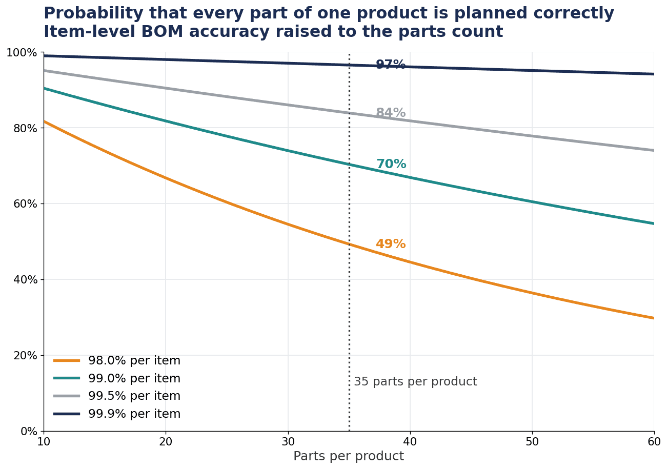
98% per item is 49% per product. Stated at item level, BOM accuracy always overstates reality
Let us unpack what the numbers mean. Raise 98.0% to the power of 35 and you get 49.3%. An item-level accuracy of 98.0%, which sounds respectable, means that on a product built from 35 parts, one product in two has a broken parts arrangement. On half of the products in the production plan, some part is either short or in surplus. That should match what the shop floor feels.
Lift it to 99.0% and the product level only reaches 70.3%. One product in three still breaks. Lift it to 99.5% and you get 83.9%, with a considerable number of products still failing. The level that holds up in practice at product level, namely 96.6%, is reached only when item-level accuracy hits 99.9%.
Two things follow from this.
First, if you are going to use item-level BOM accuracy as a target, the target can only be 99.9%. An improvement plan that says “let us aim for 98.0% first” arrives, on achievement, at a state where half the products still fail. It does not even work as an interim target. At item level, 98.0% and 99.9% look like a small difference; at product level they are 49% versus 97%, close to a doubling. The return on improvement investment is concentrated near the top of the accuracy range.
Second, the effect scales non-linearly with the number of parts in a product. At the same item accuracy of 98%, a product with 10 parts and a product with 60 parts have completely different product-level success rates. The more a factory’s part counts swell through engineer-to-order or high-mix low-volume production, the more an item-level accuracy metric overstates reality. The reason a report saying “BOM accuracy is healthy” can coexist with chaos on the shop floor is that the metric was never measuring the product-level failure rate in the first place.
Note that this calculation assumes errors occur independently. In practice there is correlation, for example when several parts tied to the same design change are wrong together, so the strict probability can come out higher than shown. Even so, the direction of the conclusion does not change. Item-level accuracy is subject to a one-way bias: it always looks better than product-level performance.
The fourth master in a Thai plant: BOI max stock and formula as a separate ledger
The three masters described so far are common to factories in any country. If your plant is in Thailand, however, there is effectively a fourth master. It is the BOI raw material ledger.
If you import raw materials duty-free using privileges from the BOI, the Thailand Board of Investment, those materials are managed for tax purposes in a framework separate from ordinary inventory. Each item has an approved max stock, the maximum quantity that may be held duty-free, and there is a formula that defines the raw material consumption per unit of product. The balance of duty-free raw material on hand is managed by deducting the consumption calculated from the formula out of the quantity imported. In other words, alongside the physical stock ledger, a second ledger for tax purposes is running.
At import clearance, too, the BOI duty exemption approval and the import declaration documents are checked against each other. A ledger that does not match reality is not merely a question of administrative precision.
What matters here is the relationship between the formula and the actual BOM. The formula is derived from BOM figures, but it is not updated with every design change the way a BOM is. When a design change alters the quantity per unit, actual raw material consumption changes, while the formula registered with the BOI does not. The BOM drift seen in the previous section propagates along the same route into a gap with this fourth ledger. A BOM drift rate of 20.0% does not translate one for one into a formula drift rate, but the property of being left unupdated is shared.
So at a Thai site, master data error takes effect through two routes. One is the production and cash route of shortages and excess stock. The other is the tax route. If the head office in Japan believes that “98% is enough for both BOM accuracy and inventory accuracy,” that is a standard which looks at only the first route.
What is happening to material procurement lead times in Thailand in 2026
We said that lead time, the third master, ages at a speed outside the company. So what is that outside speed doing in Thailand in 2026?
The Thailand Manufacturing PMI published by S&P Global stood at 54.2 in July 2026. That is up from 53.6 in June and the highest level since December 2025. Since 50 is the boundary between expansion and contraction, manufacturing activity is clearly on the expansion side.
What a buyer should read, however, is not the headline index but the breakdown. The same survey reported that purchasing activity rose at its fastest pace since March, that input delivery times lengthened, if only marginally, and that backlogs of work built up.
When those three occur together, the meaning is clear from the procurement side. Factories all around you are raising their order volumes at once, supplier backlogs are growing, and delivery times are starting to stretch as a result. The lead times registered in your master data were most likely confirmed during a period of weak demand. A turn into an expansion phase is precisely the phase in which the lead time master goes stale fastest.
In Thailand there is a further factor: a substantial share of materials is imported, so both sea freight and air freight ride on the procurement lead time. Sea freight is cheap but varies widely and is directly exposed to congestion and vessel scheduling. Air freight is fast but expensive per unit, and in practice serves as the catch-all for expedited orders. Here is the important part: when a stale lead time master causes a shortage, the fix is automatically air freight, which is to say an expedited order. A lack of master data freshness shows up every month on an invoice, in the form of transport cost.
Why a Thai site should set inventory accuracy targets higher than Japan does
Pulling the above together, there are three reasons why a site in Thailand should set its inventory accuracy and BOM accuracy targets higher than a plant in Japan.
First, error connects directly to tax risk. The BOI raw material ledger has to be consistent with physical stock, and that consistency depends on both inventory accuracy and BOM accuracy. In a Japanese plant, a stock discrepancy is processed as an inventory loss and that is the end of it; in Thailand, the reconciliation against the fourth ledger remains.
Second, recovery costs are higher. When a shortage occurs, a plant in Japan can often have a domestic supplier deliver the next day, whereas a plant in Thailand arranges air freight for imported material. The recovery cost per incident is different. At the same inventory accuracy, the monetary damage caused by the shortfall in accuracy is larger.
Third, because lead times are long, it takes longer for an error to surface. With a long procurement lead time, today’s calculation mistake shows up as a shortage several weeks later, by which time the next mistakes have already stacked up. In a system where error detection is delayed, the only real option is to raise accuracy on the input side so the error never enters.
MRP system implementation benefits and ROI: do not book the excess inventory reduction every year
Now to the return on investment. The second point we want to convey in this article concerns a calculation error that appears in almost every capital request.
Assumptions for the model factory
Let us set the assumptions first.
| Item | Value |
|---|---|
| Number of part and raw material items | 620 items |
| Average parts per product | 35 parts |
| Annual material purchase value | 57,600,000 THB |
| Daily material consumption value | 157,808 THB |
| Current material inventory | 9,600,000 THB, equal to 61 days of stock |
| Days of stock after MRP | 46 days, a reduction of 15 days |
| Inventory reduction | 2,367,000 THB, one time only |
The intermediate steps are as follows. Daily material consumption is 57,600,000 / 365 = 157,808 THB. Current days of stock is 9,600,000 / 157,808 = 60.8 days, written below as 61 days. If thinning out the safety stock buffer through MRP brings days of stock to 46, the reduction is about 15 days’ worth. The inventory reduction is 157,808 × 15 = 2,367,000 THB, rounded to the nearest thousand THB.
To repeat, this 15-day reduction does not happen automatically. It is a conditional figure: only once all three masters are trustworthy can the shop floor let go of the extra stock it holds as insurance. If you are still at the stage of comparing how to hold inventory in the first place, a comparison of factory inventory management systems is worth reading alongside this.
Breakdown of the recurring benefits
Three benefits recur every year.
| Item | Calculation | THB per year |
|---|---|---|
| Holding cost on the reduced inventory | 2,367,000 × 6% | 142,020 |
| Fewer expedited orders caused by shortages | (24 cases – 8 cases) × 38,000 THB | 608,000 |
| Less labour on requirement calculation and reconciliation | (768h – 216h) × 380 THB/h | 209,760 |
| Total recurring benefit | 959,780 |
Line one. When inventory falls by 2,367,000 THB, the cost of keeping that inventory around is saved every year: warehouse space, racking, insurance, the handling effort of receipts, issues and counting, and write-offs from deterioration and obsolescence. Taking these as 6% of inventory value, 2,367,000 × 0.06 = 142,020 THB per year. The inventory that was removed does not keep shrinking further each year, but the cost that used to be incurred every year to keep holding it stops being incurred from the following year onward. A one-time release of working capital of 2,367,000 THB and a recurring holding cost of 142,020 THB that disappears every year are two different things. This is the fork in the road for the discussion that follows.
Note that the opportunity cost of capital, the interest equivalent on working capital that had been sitting idle, is deliberately not added on top here. The released 2,367,000 THB is applied once against the initial investment, as described below. You cannot simultaneously assume that the principal pays for the investment and that the same principal earns an external return every year. That is the same pattern of double counting this article criticises, so only the holding cost is placed in the recurring benefits.
Line two. Suppose expedited orders fall from 24 cases a year to 8. If the additional cost per case, covering the switch to air freight, small-lot surcharges and internal handling effort, is 38,000 THB, then (24 – 8) × 38,000 = 608,000 THB per year. This item is the largest at the model factory, because with an imported material mix in Thailand the recovery cost of a single shortage is high.
Line three. Suppose the hours spent on manual requirement calculation and on reconciling Excel against the system fall from 768 hours a year to 216. At a labour cost of 380 THB per hour, (768 – 216) × 380 = 209,760 THB per year.
Adding them up: 142,020 + 608,000 + 209,760 = 959,780 THB per year.
The investment side is as follows.
| Item | THB |
|---|---|
| Production management system including MRP: licence and build | 2,600,000 |
| Master data preparation: BOM review and inventory accuracy start-up | 900,000 |
| Total initial investment | 3,500,000 |
| Annual maintenance | 390,000 per year |
The point worth noting is that 900,000 THB of the 3,500,000 THB initial investment is allocated to master data preparation. Given the argument of this article that allocation is only natural, but in real quotations this line is often buried inside “implementation support” and valued at zero. An implementation whose master data budget has been cut is an implementation in which only the system works correctly.
Deducting the annual maintenance of 390,000 THB, the annual net benefit is 959,780 – 390,000 = 569,780 THB per year.
The correct payback of 2.0 years and the incorrect 1.3 years
Now to the heart of the matter.
The inventory reduction of 2,367,000 THB is a one-time release of working capital. When you take stock from 61 days down to 46 days, 15 days’ worth of cash returns to you at that moment. The following year, however, inventory is already at 46 days, so it will not fall further on its own. In other words, 2,367,000 THB is a single cash receipt, not an annual benefit.
The correct treatment, therefore, is to deduct it from the initial investment.
- Effective investment = 3,500,000 – 2,367,000 = 1,133,000 THB
- Payback period = 1,133,000 / 569,780 = 2.0 years
What one frequently sees in capital requests, on the other hand, is the following calculation, in which the inventory reduction is booked as an annual benefit.
- Incorrect annual net benefit = 2,367,000 + 608,000 + 209,760 – 390,000 = 2,794,760 THB per year
- Incorrect payback period = 3,500,000 / 2,794,760 = 1.3 years
There are two reasons why this error is hard to spot. One is that the payback difference, 1.3 years against 2.0 years, keeps both inside the range of “payback in about two years.” That is not a gap that stops a review. The other is that booking the inventory reduction as an annual benefit removes the 142,020 THB holding cost line and replaces it with 2,367,000 THB, so on the surface the table can even look tidier than before.
The error grows, however, the more years pass.
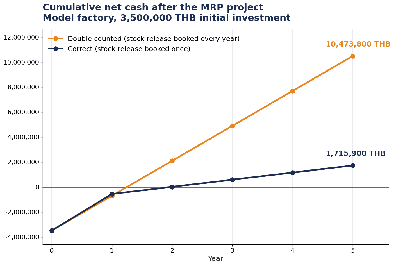
Stack the inventory reduction into the annual benefit and it swells 6.1 times over five years
Compare cumulative net cash over five years.
| Cumulative net cash over five years | |
|---|---|
| Correct calculation | 2,367,000 + 569,780 × 5 – 3,500,000 = +1,715,900 THB |
| Incorrect calculation | 2,794,760 × 5 – 3,500,000 = +10,473,800 THB |
| Difference | 8,757,900 THB, an overstatement of 6.1 times |
In the correct calculation the 2,367,000 THB from inventory reduction arrives once in the first year, after which 569,780 THB accumulates annually, giving a cumulative 1,715,900 THB. In the incorrect calculation, 2,367,000 THB is assumed to be received five times, so the cumulative figure swells to 10,473,800 THB. The difference is 8,757,900 THB, a multiple of about 6.1 times.
The reason the correct line sits higher only in year one on the chart is that the 2,367,000 THB from inventory reduction lands as a lump sum in the first year. From year two onward the incorrect calculation piles on another 2,367,000 THB every year, so it overtakes shortly after the one-year mark and the gap only widens from there.
What happens in practice? If a capital request states “MRP will deliver ten million THB of benefit over five years,” someone will have to explain that number in the year-three performance review. What the incorrect calculation promised by year three is a cumulative 4,884,280 THB. The actual cash effect at the end of year three is a cumulative plus of 576,340 THB, which is not at all bad for a figure taken just after payback is complete. Against the promise, however, it looks like barely more than a tenth. What follows is either an exercise in redefining how benefits are measured so the numbers add up, or the conclusion that “the MRP implementation was a failure.” Both occur for reasons that have nothing to do with what the system can do.
The principle for handling inventory reduction in an investment decision is simple. A change in a stock, meaning the inventory balance, happens once; a change in a flow, meaning an annual cost, is recurring. Do not mix the two in the same table and add them together. If you keep the inventory reduction as a deduction from the initial investment, there is no way for them to get mixed.
It is worth adding that the correct calculation still describes a perfectly good investment: payback in 2.0 years and a five-year cumulative plus of 1,715,900 THB. Dropping the overstatement does not change the conclusion that this is worth doing. All that changes is whether you can still explain it three years later.
Where MRP works and where it does not in engineer-to-order and high-mix low-volume production
“We are engineer-to-order, so MRP does not suit us” is something we hear often. It is half right, and half a question of how the assumptions were set.
The conditions under which MRP works can be organised as follows.
| Condition | Works when | Does not work when |
|---|---|---|
| Existence of a BOM | Component parts are fixed at the time of order receipt | Design and manufacturing run in parallel and the BOM keeps changing after work starts |
| Commonality of parts | Products differ but a substantial share of parts is common | Parts are almost entirely specific to each product |
| Procurement lead time versus delivery date | Procurement lead time is shorter than the span from order receipt to delivery | Procurement lead time is longer, so parts must be arranged before the order arrives |
| Visibility of demand | Forecasts and backlog give visibility for a certain period ahead | Nothing is known until the order arrives |
Being high-mix low-volume does not in itself determine whether MRP fits. The more variants there are, the more easily manual requirement calculation collapses, so if anything that is the case for a computer. What causes trouble is the right-hand column, especially the case where the BOM keeps changing after work starts.
Care is needed here, though. Some factories that say “our BOM never gets fixed, so MRP is impossible” simply have no business process for fixing the BOM. There is no rule for managing design changes, drawings sit on individual PCs, and reflecting them in the M-BOM is nobody’s job, and this state of affairs is explained as “we are engineer-to-order.” The two need to be diagnosed separately. The former is a discussion about changing the calculation method, for example project-based control, or a hybrid in which common parts run on MRP while product-specific parts are allocated to a project number. The latter is a discussion about designing master data operations, and changing the system will not solve it.
The relationship between procurement lead time and delivery date matters too. At a plant in Thailand, the procurement lead time for imported material frequently exceeds the span from order receipt to delivery, in which case arranging parts ahead of the order becomes unavoidable. That territory belongs not to MRP but to judgement, deciding advance order quantities from forecast information and past results. Holding common parts on a forecast basis and exploding product-specific parts with MRP after order receipt is a realistic two-tier answer. Apply MRP to every item without designing that split, and all you are left with is the impression that “the calculation results do not match reality.”
How to run the implementation: designing operations that keep master data fresh
Let us return to the drift table at the beginning. BOM 20.0%, inventory 11.9%, lead time and order lot 78.1%. Building a mechanism that keeps these three numbers low after go-live is what an MRP implementation project actually consists of.
Assign an owner and an update frequency to each master
The first thing to do is extremely administrative: for each of the three masters, write down and decide the update trigger, the owner, the frequency, and the measurement method.
| Master | Update trigger | What has to be decided | Metric |
|---|---|---|---|
| Bill of materials (BOM) | Issue of a design change | Who reflects the E-BOM change into the M-BOM and by when, and how completion is confirmed | Ratio of unreflected changes to total design changes |
| Inventory | Every receipt and issue | Timing of record entry, and when reconciliation against the physical item takes place | Rate of items with discrepancies in cycle counting |
| Lead time and order lot | Supplier notification, or a gap against actual performance | Who receives supplier changes, and when they are reflected in the master | Ratio of unreflected changes to total changes |
The third row is what stays blank in most factories. Filling it in alone brings the 78.1% drift rate down substantially. The method is not difficult: aggregate actual lead times automatically from order and receipt records, list monthly those items whose gap against the master value exceeds a threshold, and have the buyer review them. A mechanism of roughly that scale is enough to give an internal update cycle to a master that ages at an external speed.
If you are designing this together with the ordering process itself, organising order and purchasing management systems is a useful reference.
One more point deserves emphasis: what it means to decide on a metric. While drift rates go unmeasured, master data decay is invisible to management, and what is invisible does not become a target for improvement. Changing how you measure the success of an MRP implementation, from “is the system running” to “what percentage are the three drift rates,” is the real substance of operational design.
Measure inventory accuracy daily with cycle counting
For the inventory master, an annual physical count cannot preserve freshness. From the day after the count until the next one, inventory accuracy keeps decaying without being measured.
Cycle counting is used instead. Rather than counting every item at once, you count a small number of items every day and cycle through the whole item list over a set period. With the model factory’s 620 items, counting just a few items a day is enough to cover every item several times a year. The practical advantages are that the line does not have to stop and that it can be embedded as a daily task.
The essence of cycle counting is not aligning inventory but finding the cause of discrepancies every day. Even if an annual count turns up 74 items with discrepancies, you cannot trace when or why each one arose. Count daily and, for any item showing a discrepancy, you can trace “which recent receipts and issues are involved” and identify whether it was a missed entry, a wrong storage location, or an over-issue caused by a wrong quantity per unit. That last case is in fact a BOM error surfacing as an inventory discrepancy. The three masters are not independent; this is how they expose each other’s errors.
If you want to set priorities, count high-value items and fast-moving items more frequently. There is no need to treat all 620 items at the same frequency.
Frequently asked questions (FAQ)
What is the difference between an MRP system, an ERP and a production management system?
MRP is the name of a function, while ERP and production management system are names of product categories. MRP refers to “the function that calculates the quantity and timing of required materials,” and it is implemented as part of many production management systems and ERPs. A comparison framed as “should we choose an MRP system or an ERP” therefore does not really hold. What should be examined is whether the MRP function of the production management system or ERP you select supports your production model, such as make-to-stock or make-to-order and whether project-based control is required, and whether it can be placed on an operation that maintains the three masters.
What does an MRP system cost?
At the scale of the model factory, with 620 part and raw material items, the structure is 2,600,000 THB for licence and build, 900,000 THB for master data preparation, 3,500,000 THB of initial investment in total, and 390,000 THB of annual maintenance. Since the figures move with item count, number of sites and the scope of integration with existing systems, please read them as an indication of order of magnitude. What matters more than the total is the breakdown. A quotation with no budget line for master data preparation means the cost of managing drift rates after go-live sits in nobody’s budget.
Can material requirements planning be done in Excel?
The calculation itself is possible. Many factories do in fact explode requirements in Excel. The problem is not computing power but whether you can keep maintaining updates to the three masters in Excel. In an environment with 210 design changes a year, when the BOM sheet is updated by hand and several people hold separate files, drift rates can only move upward. The model factory was spending 768 hours a year on requirement calculation and reconciliation. The deciding factor is that workload, together with whether you can sustain single-source master data management manually.
What level of inventory accuracy makes MRP usable?
No answer can be given from inventory accuracy alone, because the correctness of MRP output is the product of inventory, BOM and lead time. A way of thinking can still be offered. On BOM accuracy, obtaining a product-level success rate of 96.6% on a product built from 35 parts required 99.9% at item level. The same direction of bias applies to inventory. That said, raising the stocktaking discrepancy rate to the power of the part count is excessive, because discrepancies cluster in particular items and storage locations, so the assumption of independence does not hold. Even so, it is certain that the model factory’s inventory discrepancy level of 11.9% affects the arrangement of far more products than the item-level impression suggests. Realistically, the target is to switch from aligning things at an annual count to measuring the discrepancy rate routinely through cycle counting, and then to keep driving that metric down.
How does a stockout prevention system differ from MRP?
Most mechanisms aimed at preventing stockouts are reorder point systems. They are reactive: order when stock falls below a set level. The settings are simple and the method is easy to operate, but it cannot notice when the stock figure it reads diverges from reality. MRP is predictive, calculating future requirements from the production plan, and it is strong when demand variation is known in advance. The two are not exclusive. In practice, using reorder point control for fast-moving, inexpensive common parts and MRP for high-value parts tied to the plan is a workable split. Both, however, take the same masters as input, so if the masters are stale, both will miss.
Summary
The reason an MRP system does not run is neither the calculation engine nor the product selection; it is the freshness of the master data on the input side. To recap the key points.
- The inputs to MRP are on-hand stock, the bill of materials (BOM), and lead time and order lot, and the correctness of the output is the product of the three
- The three age at different speeds. The BOM at the speed of design change, a drift rate of 20.0%; inventory at the speed of every working day, 11.9%; lead time and order lot at a speed outside the company, 78.1%. The most neglected is the third, the one with no assigned owner for updates
- Stated at item level, BOM accuracy always overstates reality. On a product built from 35 parts, 98.0% per item is 49% per product, 99.0% gives 70%, and 99.5% gives 84%. The practical level of 97% is reached only at 99.9% per item
- A Thai site has a fourth ledger in the BOI max stock and formula, so inventory and BOM error takes effect through the tax route as well. The PMI for July 2026 was 54.2, an expansion phase, input delivery times are lengthening, and this is the period in which the lead time master goes stale fastest
- In an ROI estimate, the inventory reduction of 2,367,000 THB is a one-time release of working capital and is deducted from the initial investment. The correct payback is 2.0 years; the error of booking it as an annual benefit gives 1.3 years. The difference looks small, but over five years the cumulative figures are 1,715,900 THB against 10,473,800 THB, a gap of 6.1 times
- The real substance of an implementation project is assigning an update owner, an update frequency and a metric to each of the three masters, and for inventory, building an operation that measures daily through cycle counting
And once more at the end: installing MRP does not by itself reduce inventory. Inventory falls only when, as a result of the master data becoming correct, the shop floor can let go of the stock it holds as insurance.
TOMAS TECH supports Japanese-affiliated manufacturers in Thailand in building production and inventory management practices. We also welcome enquiries at the stage before an implementation decision is made, such as “we would like to measure how stale our own three masters are right now” or “we would like a third party to look at whether the benefit calculation in our capital request is set up correctly.” Even if you are only starting to organise the current issues, please feel free to get in touch via our contact page.
References
- S&P Global Thailand Manufacturing PMI, July 2026
- News coverage of the Thailand manufacturing PMI, August 2026
- BOM design decides whether a production management system succeeds
- The bill of materials (BOM) and the difference between E-BOM and M-BOM
- Formulas for optimal stock, safety stock and cycle stock
- The paradox of running out of parts while holding excess inventory
- Import clearance procedures when using BOI duty exemption measures, JETRO
- Making parts procurement more efficient with the bill of materials (BOM)